Fitting curves to real data
Overview
When you have a real dataset, the easiest way to fit it is via the neutcurve.curvefits.CurveFits class, which streamlines the fitting and plotting of a set of neutcurve.hillcurve.HillCurve neutralization curves. Here we demonstrate how to do this.
Importing Python packages
First, import the necessary Python modules. In addition to the neutcurve package itself, we also use pandas to hold the data:
[1]:
import pandas as pd

import neutcurve
from neutcurve.colorschemes import CBMARKERS, CBPALETTE
Set some pandas display options:
[2]:
pd.set_option("display.float_format", "{:.3g}".format)
pd.set_option("display.max_columns", 20)
pd.set_option("display.width", 500)
Preparing the data
Now we get example data to fit. We use as our example the neutralization of variants A/WSN/1933 (H1N1) influenza by the broadly neutralizing antibody FI6v3 and strain-specific antibody H17-L19 from Fig 6a,b of Doud et al (2018). We start by reading these data into a pandas DataFrame:
[3]:
fi6v3_datafile = "Doud_et_al_2018-neutdata.csv"
[4]:
data = pd.read_csv(fi6v3_datafile)

# drop replicate 2 for one serum as this helps with some plot testing below
data = data[(data["serum"] != "H17-L19") | (data["replicate"] != 2)]
Here are the first few lines of the data frame:
[5]:
data.head()
[5]:
| serum | virus | replicate | concentration | fraction infectivity | |
|---|---|---|---|---|---|
| 0 | FI6v3 | WT | 1 | 0.000205 | 1.01 |
| 1 | FI6v3 | WT | 1 | 0.000478 | 0.942 |
| 2 | FI6v3 | WT | 1 | 0.00112 | 0.993 |
| 3 | FI6v3 | WT | 1 | 0.0026 | 0.966 |
| 4 | FI6v3 | WT | 1 | 0.00607 | 0.957 |
And here are the last few lines:
[6]:
data.tail()
[6]:
| serum | virus | replicate | concentration | fraction infectivity | |
|---|---|---|---|---|---|
| 427 | H17-L19 | V135T | 3 | 0.386 | 1.02 |
| 428 | H17-L19 | V135T | 3 | 0.9 | 1 |
| 429 | H17-L19 | V135T | 3 | 2.1 | 0.959 |
| 430 | H17-L19 | V135T | 3 | 4.9 | 0.991 |
| 431 | H17-L19 | V135T | 3 | 11.4 | 0.747 |
As can be seen above, the data are organized into five columns, all of which must be present. These columns are:
serum: the name of the serum (or antibody). FI6v3 and H17-L19 are actually antibodies, not sera, but
neutcurve.curvefits.CurveFitsis set up to refer to things as serum.virus: the name of the virus being neutralized by the serum.
replicate: the replicate label for the measurement. Although you can have just one replicate, it’s good experimental practice to have several. All the replicates for a given virus / serum combination must have been measured at the same concentrations.
concentration: the concentration of the serum.
fraction infectivity: the fraction infectivity of the virus at this concentration of the serum measured in this replicate.
Note that the data are in tidy form; you must make your data frame tidy before you can analyze it with neutcurve.curvefits.CurveFits.
Fitting the curves
Once you have the tidy data frame, it’s easy to pass it to neutcurve.curvefits.CurveFits. We expect all of these antibodies to go to complete neutralization when they are effective, so we use default values of and argument (see neutcurve.hillcurve.HillCurves and Hill-curve neutralization for more details about the and options):
[7]:
fits = neutcurve.CurveFits(data)
Now we can look at the different sera for which we have fit curves:
[8]:
fits.sera
[8]:
['FI6v3', 'H17-L19']
We can also look at the viruses measured against each serum:
[9]:
for serum in fits.sera:
    print(f"Viruses measured against {serum}:\n" + str(fits.viruses[serum]))
Viruses measured against FI6v3:
['WT', 'K(-8T)', 'P80D', 'V135T', 'K280A', 'K280S', 'K280T', 'N291S', 'M17L-HA2', 'G47R-HA2']
Viruses measured against H17-L19:
['WT', 'V135T']
We can also look at the replicates for each serum and virus. Here we just do that for serum FI6v3 and virus WT. See how in addition to the three replicates we have passed, there is also now an “average” replicate that is automatically computed from the average of the other replicates:
[10]:
fits.replicates[("FI6v3", "WT")]
[10]:
['1', '2', '3', 'average']
Looking at a specific curve
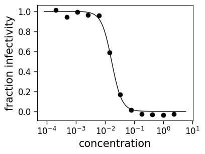
We can use the neutcurve.curvefits.CurveFits.getCurve() method to get the neutcurve.hillcurve.HillCurve that was fit for a particular serum / virus / replicate combination. For instance, here we do that for serum FI6v3 versus virus WT for replicate 1. We then plot the curve and print the IC50:
[11]:
curve = fits.getCurve(serum="FI6v3", virus="WT", replicate="1")
print(f"The IC50 is {curve.ic50():.3g}")
fig, ax = curve.plot()
The IC50 is 0.0167
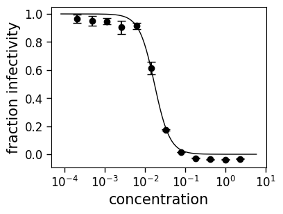
neutcurve.curvefits.CurveFits also calculates the average and standard error of the measurements for each serum / virus, and fits them under a replicate name of “average”. Here is the fit to the average of the data for serum FI6v3 and virus WT. Note how the plot now also shows error bars indicating the standard error:
[12]:
curve = fits.getCurve(serum="FI6v3", virus="WT", replicate="average")
print(f"The IC50 is {curve.ic50():.3g}")
fig, ax = curve.plot()
The IC50 is 0.017
Accessing the fit parameters for all curves
You can get the fit parameters for the curves using neutcurve.curvefits.CurveFits.fitParams(). By default, this just gets the fits for the average of the replicates. The parameters are all of those fit by a neutcurve.hillcurve.HillCurve, plus the IC50 in several forms to accurately represent interpolated IC50s (IC50 within range of data) versus IC50s where we can just get the bound from the upper or lower limits of the data:
[13]:
fits.fitParams()
[13]:
| serum | virus | replicate | nreplicates | ic50 | ic50_bound | ic50_str | midpoint | midpoint_bound | midpoint_bound_type | slope | top | bottom | r2 | rmsd | |
|---|---|---|---|---|---|---|---|---|---|---|---|---|---|---|---|
| 0 | FI6v3 | WT | average | 3 | 0.017 | interpolated | 0.017 | 0.017 | 0.017 | interpolated | 2.28 | 1 | 0 | 0.992 | 0.0389 |
| 1 | FI6v3 | K(-8T) | average | 3 | 0.0283 | interpolated | 0.0283 | 0.0283 | 0.0283 | interpolated | 2.4 | 1 | 0 | 0.986 | 0.0592 |
| 2 | FI6v3 | P80D | average | 3 | 0.0123 | interpolated | 0.0123 | 0.0123 | 0.0123 | interpolated | 2.05 | 1 | 0 | 0.99 | 0.0467 |
| 3 | FI6v3 | V135T | average | 3 | 0.0229 | interpolated | 0.0229 | 0.0229 | 0.0229 | interpolated | 1.83 | 1 | 0 | 0.995 | 0.0328 |
| 4 | FI6v3 | K280A | average | 3 | 0.0106 | interpolated | 0.0106 | 0.0106 | 0.0106 | interpolated | 1.86 | 1 | 0 | 0.981 | 0.0655 |
| 5 | FI6v3 | K280S | average | 3 | 0.0428 | interpolated | 0.0428 | 0.0428 | 0.0428 | interpolated | 2 | 1 | 0 | 0.993 | 0.0376 |
| 6 | FI6v3 | K280T | average | 3 | 0.0348 | interpolated | 0.0348 | 0.0348 | 0.0348 | interpolated | 1.82 | 1 | 0 | 0.993 | 0.0375 |
| 7 | FI6v3 | N291S | average | 3 | 0.0845 | interpolated | 0.0845 | 0.0845 | 0.0845 | interpolated | 1.8 | 1 | 0 | 0.997 | 0.0228 |
| 8 | FI6v3 | M17L-HA2 | average | 3 | 0.0198 | interpolated | 0.0198 | 0.0198 | 0.0198 | interpolated | 2.06 | 1 | 0 | 0.989 | 0.0483 |
| 9 | FI6v3 | G47R-HA2 | average | 3 | 0.0348 | interpolated | 0.0348 | 0.0348 | 0.0348 | interpolated | 2.6 | 1 | 0 | 0.982 | 0.0674 |
| 10 | H17-L19 | WT | average | 2 | 0.106 | interpolated | 0.106 | 0.106 | 0.106 | interpolated | 4.04 | 1 | 0 | 0.99 | 0.0518 |
| 11 | H17-L19 | V135T | average | 2 | 11.4 | lower | >11.4 | 16.9 | 11.4 | lower | 2.36 | 1 | 0 | 0.708 | 0.052 |
Looking above, you can see how the IC50 is handled depending on if it is interpolated (in the range of concentrations used in the experiments) versus outside the range of concentrations. In the table above, all of the IC50s are interpolated except the last row (H17-L19 versus V135T), which is just provided as an upper bound equal to the highest concentration used in the experiment (the actual IC50 is greater than this upper bound). We do not attempt to extrapolate IC50s outside the data range as this is unreliable.
You can see there is also a column (“r2”) that reports the coefficient of determination as a measure of how well the curve fits the data.
Note that by default, neutcurve.curvefits.CurveFits.fitParams() only returns the fitted params for the averages, as in the above table. If you want to also return them for individual replicates, using argument average_only=False. Here we do this, showing only the first few entries in the returned data frame; now there are now values for each replicate as well as the average of replicates:
[14]:
fits.fitParams(average_only=False).head()
[14]:
| serum | virus | replicate | nreplicates | ic50 | ic50_bound | ic50_str | midpoint | midpoint_bound | midpoint_bound_type | slope | top | bottom | r2 | rmsd | |
|---|---|---|---|---|---|---|---|---|---|---|---|---|---|---|---|
| 0 | FI6v3 | WT | 1 | <NA> | 0.0167 | interpolated | 0.0167 | 0.0167 | 0.0167 | interpolated | 2.5 | 1 | 0 | 0.996 | 0.0284 |
| 1 | FI6v3 | WT | 2 | <NA> | 0.019 | interpolated | 0.019 | 0.019 | 0.019 | interpolated | 2.51 | 1 | 0 | 0.986 | 0.0527 |
| 2 | FI6v3 | WT | 3 | <NA> | 0.0152 | interpolated | 0.0152 | 0.0152 | 0.0152 | interpolated | 1.88 | 1 | 0 | 0.982 | 0.0597 |
| 3 | FI6v3 | WT | average | 3 | 0.017 | interpolated | 0.017 | 0.017 | 0.017 | interpolated | 2.28 | 1 | 0 | 0.992 | 0.0389 |
| 4 | FI6v3 | K(-8T) | 1 | <NA> | 0.0308 | interpolated | 0.0308 | 0.0308 | 0.0308 | interpolated | 2.62 | 1 | 0 | 0.977 | 0.077 |
The “average” is the curve fit to the average of the data points, not the average of the fit parameters for individual curves.
You can also use no_average to not show the average:
[15]:
fits.fitParams(average_only=False, no_average=True).head()
[15]:
| serum | virus | replicate | nreplicates | ic50 | ic50_bound | ic50_str | midpoint | midpoint_bound | midpoint_bound_type | slope | top | bottom | r2 | rmsd | |
|---|---|---|---|---|---|---|---|---|---|---|---|---|---|---|---|
| 0 | FI6v3 | WT | 1 | <NA> | 0.0167 | interpolated | 0.0167 | 0.0167 | 0.0167 | interpolated | 2.5 | 1 | 0 | 0.996 | 0.0284 |
| 1 | FI6v3 | WT | 2 | <NA> | 0.019 | interpolated | 0.019 | 0.019 | 0.019 | interpolated | 2.51 | 1 | 0 | 0.986 | 0.0527 |
| 2 | FI6v3 | WT | 3 | <NA> | 0.0152 | interpolated | 0.0152 | 0.0152 | 0.0152 | interpolated | 1.88 | 1 | 0 | 0.982 | 0.0597 |
| 3 | FI6v3 | K(-8T) | 1 | <NA> | 0.0308 | interpolated | 0.0308 | 0.0308 | 0.0308 | interpolated | 2.62 | 1 | 0 | 0.977 | 0.077 |
| 4 | FI6v3 | K(-8T) | 2 | <NA> | 0.0284 | interpolated | 0.0284 | 0.0284 | 0.0284 | interpolated | 2.55 | 1 | 0 | 0.986 | 0.0601 |
We can also include arbitrary inhibitory concentrations, such as the IC95 in addition to the IC50 via the argument toneutcurve.curvefits.CurveFits.fitParams(). For instance:
[16]:
fits.fitParams(ics=[50, 95])
[16]:
| serum | virus | replicate | nreplicates | ic50 | ic50_bound | ic50_str | ic95 | ic95_bound | ic95_str | midpoint | midpoint_bound | midpoint_bound_type | slope | top | bottom | r2 | rmsd | |
|---|---|---|---|---|---|---|---|---|---|---|---|---|---|---|---|---|---|---|
| 0 | FI6v3 | WT | average | 3 | 0.017 | interpolated | 0.017 | 0.062 | interpolated | 0.062 | 0.017 | 0.017 | interpolated | 2.28 | 1 | 0 | 0.992 | 0.0389 |
| 1 | FI6v3 | K(-8T) | average | 3 | 0.0283 | interpolated | 0.0283 | 0.0967 | interpolated | 0.0967 | 0.0283 | 0.0283 | interpolated | 2.4 | 1 | 0 | 0.986 | 0.0592 |
| 2 | FI6v3 | P80D | average | 3 | 0.0123 | interpolated | 0.0123 | 0.0516 | interpolated | 0.0516 | 0.0123 | 0.0123 | interpolated | 2.05 | 1 | 0 | 0.99 | 0.0467 |
| 3 | FI6v3 | V135T | average | 3 | 0.0229 | interpolated | 0.0229 | 0.114 | interpolated | 0.114 | 0.0229 | 0.0229 | interpolated | 1.83 | 1 | 0 | 0.995 | 0.0328 |
| 4 | FI6v3 | K280A | average | 3 | 0.0106 | interpolated | 0.0106 | 0.0516 | interpolated | 0.0516 | 0.0106 | 0.0106 | interpolated | 1.86 | 1 | 0 | 0.981 | 0.0655 |
| 5 | FI6v3 | K280S | average | 3 | 0.0428 | interpolated | 0.0428 | 0.186 | interpolated | 0.186 | 0.0428 | 0.0428 | interpolated | 2 | 1 | 0 | 0.993 | 0.0376 |
| 6 | FI6v3 | K280T | average | 3 | 0.0348 | interpolated | 0.0348 | 0.176 | interpolated | 0.176 | 0.0348 | 0.0348 | interpolated | 1.82 | 1 | 0 | 0.993 | 0.0375 |
| 7 | FI6v3 | N291S | average | 3 | 0.0845 | interpolated | 0.0845 | 0.433 | interpolated | 0.433 | 0.0845 | 0.0845 | interpolated | 1.8 | 1 | 0 | 0.997 | 0.0228 |
| 8 | FI6v3 | M17L-HA2 | average | 3 | 0.0198 | interpolated | 0.0198 | 0.083 | interpolated | 0.083 | 0.0198 | 0.0198 | interpolated | 2.06 | 1 | 0 | 0.989 | 0.0483 |
| 9 | FI6v3 | G47R-HA2 | average | 3 | 0.0348 | interpolated | 0.0348 | 0.108 | interpolated | 0.108 | 0.0348 | 0.0348 | interpolated | 2.6 | 1 | 0 | 0.982 | 0.0674 |
| 10 | H17-L19 | WT | average | 2 | 0.106 | interpolated | 0.106 | 0.221 | interpolated | 0.221 | 0.106 | 0.106 | interpolated | 4.04 | 1 | 0 | 0.99 | 0.0518 |
| 11 | H17-L19 | V135T | average | 2 | 11.4 | lower | >11.4 | 11.4 | lower | >11.4 | 16.9 | 11.4 | lower | 2.36 | 1 | 0 | 0.708 | 0.052 |
Include standard deviations on IC50s calculated from estimated errors on parameters during fitting. Note that although this method is implemented, we strongly recommend instead fitting each replicate separately and computing errors that way instead (see immediately below):
[17]:
fits.fitParams(ic50_error="fit_stdev")
[17]:
| serum | virus | replicate | nreplicates | ic50 | ic50_bound | ic50_str | ic50_error | midpoint | midpoint_bound | midpoint_bound_type | slope | top | bottom | r2 | rmsd | |
|---|---|---|---|---|---|---|---|---|---|---|---|---|---|---|---|---|
| 0 | FI6v3 | WT | average | 3 | 0.017 | interpolated | 0.017 | 0.0254 | 0.017 | 0.017 | interpolated | 2.28 | 1 | 0 | 0.992 | 0.0389 |
| 1 | FI6v3 | K(-8T) | average | 3 | 0.0283 | interpolated | 0.0283 | 0.0411 | 0.0283 | 0.0283 | interpolated | 2.4 | 1 | 0 | 0.986 | 0.0592 |
| 2 | FI6v3 | P80D | average | 3 | 0.0123 | interpolated | 0.0123 | 0.0193 | 0.0123 | 0.0123 | interpolated | 2.05 | 1 | 0 | 0.99 | 0.0467 |
| 3 | FI6v3 | V135T | average | 3 | 0.0229 | interpolated | 0.0229 | 0.0382 | 0.0229 | 0.0229 | interpolated | 1.83 | 1 | 0 | 0.995 | 0.0328 |
| 4 | FI6v3 | K280A | average | 3 | 0.0106 | interpolated | 0.0106 | 0.0176 | 0.0106 | 0.0106 | interpolated | 1.86 | 1 | 0 | 0.981 | 0.0655 |
| 5 | FI6v3 | K280S | average | 3 | 0.0428 | interpolated | 0.0428 | 0.0683 | 0.0428 | 0.0428 | interpolated | 2 | 1 | 0 | 0.993 | 0.0376 |
| 6 | FI6v3 | K280T | average | 3 | 0.0348 | interpolated | 0.0348 | 0.0582 | 0.0348 | 0.0348 | interpolated | 1.82 | 1 | 0 | 0.993 | 0.0375 |
| 7 | FI6v3 | N291S | average | 3 | 0.0845 | interpolated | 0.0845 | 0.142 | 0.0845 | 0.0845 | interpolated | 1.8 | 1 | 0 | 0.997 | 0.0228 |
| 8 | FI6v3 | M17L-HA2 | average | 3 | 0.0198 | interpolated | 0.0198 | 0.0313 | 0.0198 | 0.0198 | interpolated | 2.06 | 1 | 0 | 0.989 | 0.0483 |
| 9 | FI6v3 | G47R-HA2 | average | 3 | 0.0348 | interpolated | 0.0348 | 0.0477 | 0.0348 | 0.0348 | interpolated | 2.6 | 1 | 0 | 0.982 | 0.0674 |
| 10 | H17-L19 | WT | average | 2 | 0.106 | interpolated | 0.106 | 0.144 | 0.106 | 0.106 | interpolated | 4.04 | 1 | 0 | 0.99 | 0.0518 |
| 11 | H17-L19 | V135T | average | 2 | 11.4 | lower | >11.4 | NaN | 16.9 | 11.4 | lower | 2.36 | 1 | 0 | 0.708 | 0.052 |
Here is the recommended way to get error estimates by just taking the average of fits for each replicate:
[18]:
params_avg_fit = fits.fitParams()[
    ["serum", "virus", "ic50", "ic50_bound", "nreplicates"]
]
params_avg_reps = (
    fits.fitParams(average_only=False)
    .query('replicate != "average"')
    .groupby(["serum", "virus"])
    .aggregate(
        ic50_replicate_avg=pd.NamedAgg("ic50", "mean"),
        ic50_replicate_stderr=pd.NamedAgg("ic50", "sem"),
    )
    .reset_index()
)
params_avg_fit.merge(params_avg_reps, on=["serum", "virus"])
[18]:
| serum | virus | ic50 | ic50_bound | nreplicates | ic50_replicate_avg | ic50_replicate_stderr | |
|---|---|---|---|---|---|---|---|
| 0 | FI6v3 | WT | 0.017 | interpolated | 3 | 0.017 | 0.00112 |
| 1 | FI6v3 | K(-8T) | 0.0283 | interpolated | 3 | 0.0283 | 0.0015 |
| 2 | FI6v3 | P80D | 0.0123 | interpolated | 3 | 0.0123 | 0.000271 |
| 3 | FI6v3 | V135T | 0.0229 | interpolated | 3 | 0.0229 | 0.000201 |
| 4 | FI6v3 | K280A | 0.0106 | interpolated | 3 | 0.0106 | 0.000819 |
| 5 | FI6v3 | K280S | 0.0428 | interpolated | 3 | 0.0428 | 0.000821 |
| 6 | FI6v3 | K280T | 0.0348 | interpolated | 3 | 0.0349 | 0.00155 |
| 7 | FI6v3 | N291S | 0.0845 | interpolated | 3 | 0.0844 | 0.00448 |
| 8 | FI6v3 | M17L-HA2 | 0.0198 | interpolated | 3 | 0.0197 | 0.000986 |
| 9 | FI6v3 | G47R-HA2 | 0.0348 | interpolated | 3 | 0.0347 | 0.000766 |
| 10 | H17-L19 | WT | 0.106 | interpolated | 2 | 0.107 | 0.012 |
| 11 | H17-L19 | V135T | 11.4 | lower | 2 | 11.4 | 0 |
Plotting the curves
One of the most useful feature of neutcurve.curvefits.CurveFits are that they have methods to easily generate multi-panel plots of the curves.
Plotting each serum against multiple viruses
Often you will have measured each serum against several different viral variants. You can then plot these curves using neutcurve.curvefits.CurveFits.plotSera() as below:
[19]:
fig, axes = fits.plotSera(xlabel="concentration (ug/ml)")
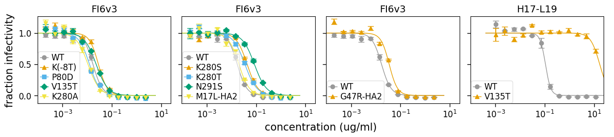
The above plot attempts to put all the viruses measured against each serum on the same subplot, but is cognizant of the fact that it becomes uninterpretable if there are too many viruses on the same plot. Therefore, it only shows a maximum of (which by default is 5) curves per subplot.
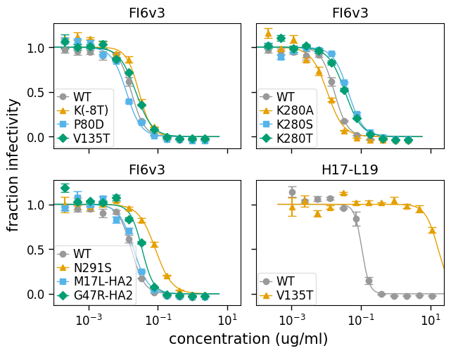
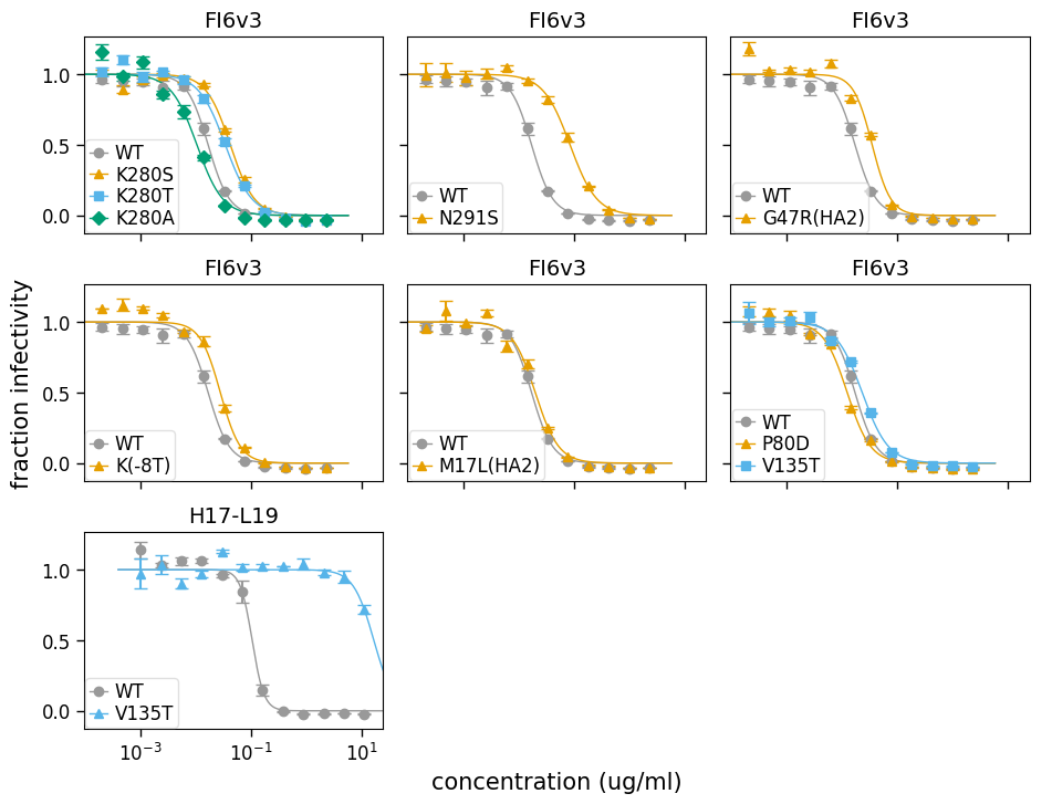
In fact, that is still perhaps too many curves per plot for this data set. So we can customize the plot by adjusting that parameter. Below we adjust to just four viruses per subplot, and also use to specify that we want two columns:
[20]:
fig, axes = fits.plotSera(
    max_viruses_per_subplot=4, ncol=2, xlabel="concentration (ug/ml)"
)
And here is plotting only the line in bounds of the data points using draw_in_bounds=True:
[21]:
fig, axes = fits.plotSera(
    max_viruses_per_subplot=4,
    ncol=2,
    xlabel="concentration (ug/ml)",
    draw_in_bounds=True,
)

The above plots all have a different legend for each subplot. This is necessary because the number of different viruses being plotted exceeds the numbers of colors / markers specified to neutcurve.curvefits.CurveFits.plotSera() via its and arguments, so there aren’t enough colors / markers to give each virus a unique one.
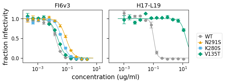
However, if we reduce the number of viruses we are showing, we then get a nice shared legend. Here we do this, using the argument to specify that we just show some of the viruses:
[22]:
fig, axes = fits.plotSera(
    viruses=["WT", "N291S", "K280S", "V135T"], xlabel="concentration (ug/ml)"
)
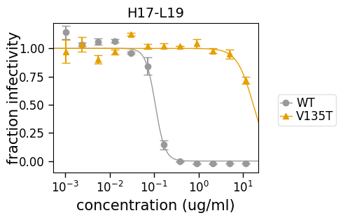
Similar to how the above plot uses the argument to plot just some viruses, we can also use the argument to plot just some of the sera (in this case, just H17-L19):
[23]:
fig, axes = fits.plotSera(sera=["H17-L19"], xlabel="concentration (ug/ml)")
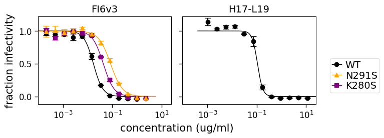
We can also use the argument to specify a particular color scheme:
[24]:
fig, axes = fits.plotSera(
    viruses=["WT", "N291S", "K280S"],
    xlabel="concentration (ug/ml)",
    virus_to_color_marker={
        "WT": ("black", "o"),
        "N291S": ("orange", "^"),
        "K280S": ("purple", "s"),
    },
    legendfontsize=14,
)
There are various additional options to neutcurve.curvefits.CurveFits.plotSera() that can further fine-tune the plots; see the docstring for that method for more details.
Plotting each virus against multiple sera
It is also possible to plot each virus against multiple sera using neutcurve.curvefits.CurveFits.plotViruses() as below:
[25]:
fig, axes = fits.plotViruses(xlabel="concentration (ug/ml)")
We can also make the plot for just certain viruses:
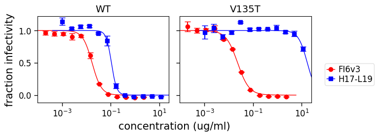
[26]:
fig, axes = fits.plotViruses(
    xlabel="concentration (ug/ml)",
    viruses=["WT", "V135T"],
    serum_to_color_marker={"FI6v3": ("red", "o"), "H17-L19": ("blue", "s")},
)
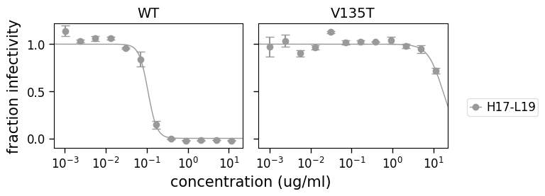
and also for just certain sera:
[27]:
fig, axes = fits.plotViruses(
    xlabel="concentration (ug/ml)", viruses=["WT", "V135T"], sera=["H17-L19"]
)
Plotting each replicate
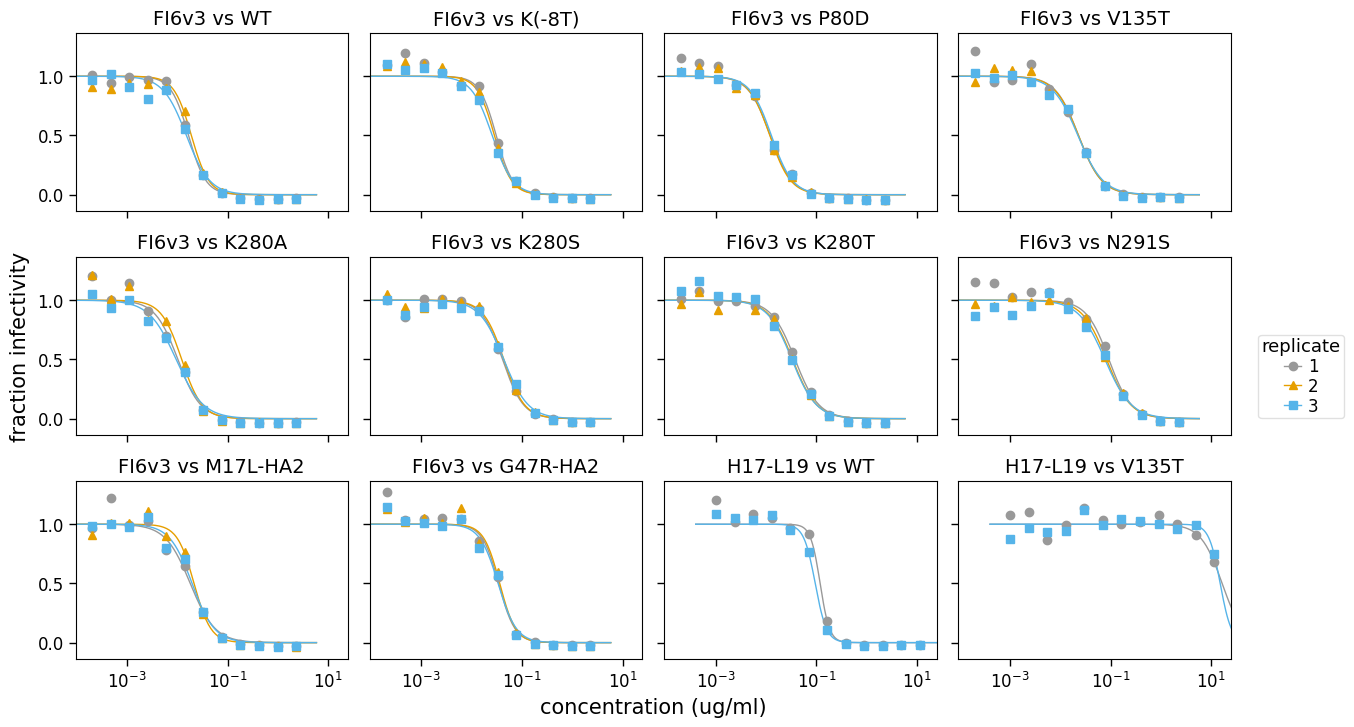
Another type of plot that is sometimes useful is one that shows all the replicates for each serum / virus combination. Such a plot is easily generated using neutcurve.curvefits.CurveFits.plotReplicates() as below:
[28]:
fig, axes = fits.plotReplicates(xlabel="concentration (ug/ml)", legendtitle="replicate")
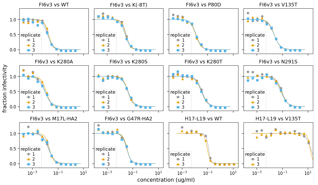
If you do not want to share the legend across panesl, use attempt_shared_legend=False:
[29]:
fig, axes = fits.plotReplicates(
    xlabel="concentration (ug/ml)",
    legendtitle="replicate",
    attempt_shared_legend=False,
)
See the method docstring for neutcurve.curvefits.CurveFits.plotReplicates() for ways to further customize these plots.
Plotting average for each serum-virus pair
Another type of plot that is useful is one that simply shows the replicate-average for each serum-virus pair on its own subplot. This plot can be generated with neutcurve.curvefits.CurveFits.plotAverages():
[30]:
fig, axes = fits.plotAverages(xlabel="concentration (ug/ml)")
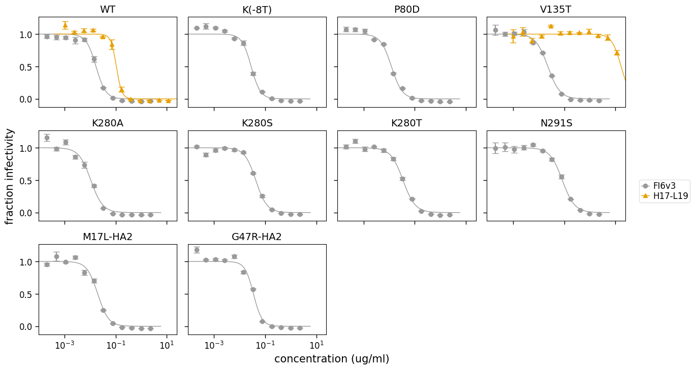
Customized plot arrangements
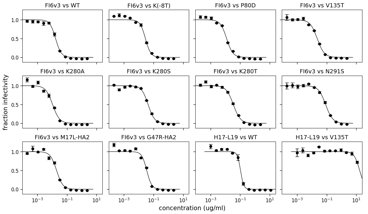
There are obviously many other ways that it’s possible to lay out the different curves for sera / viruses / replicates on subplots. You can make an arbitrarily customized layout using neutcurve.curvefits.CurveFits.plotGrid() where you explicitly pass the curves to put at each subplot in the plot.
Below we illustrate how to do this to create a plot that essentially mimics what is shown in Fig 6a,b of Doud et al (2018) (although those published plots were not generated using this program). Note that in doing this below, we use the colors and markers defined by and in neutcurve.colorschemes:
[31]:
fig, axes = fits.plotGrid(
    {
        # upper right: FI6v3 versus WT, K280S, K280T, K280A
        (0, 0): (
            "FI6v3",
            [
                {
                    "serum": "FI6v3",
                    "virus": "WT",
                    "replicate": "average",
                    "color": CBPALETTE[0],
                    "marker": CBMARKERS[0],
                    "label": "WT",
                },
                {
                    "serum": "FI6v3",
                    "virus": "K280S",
                    "replicate": "average",
                    "color": CBPALETTE[1],
                    "marker": CBMARKERS[1],
                    "label": "K280S",
                },
                {
                    "serum": "FI6v3",
                    "virus": "K280T",
                    "replicate": "average",
                    "color": CBPALETTE[2],
                    "marker": CBMARKERS[2],
                    "label": "K280T",
                },
                {
                    "serum": "FI6v3",
                    "virus": "K280A",
                    "replicate": "average",
                    "color": CBPALETTE[3],
                    "marker": CBMARKERS[3],
                    "label": "K280A",
                },
            ],
        ),
        # upper center: FI6v3 versus WT, N291S
        (0, 1): (
            "FI6v3",
            [
                {
                    "serum": "FI6v3",
                    "virus": "WT",
                    "replicate": "average",
                    "color": CBPALETTE[0],
                    "marker": CBMARKERS[0],
                    "label": "WT",
                },
                {
                    "serum": "FI6v3",
                    "virus": "N291S",
                    "replicate": "average",
                    "color": CBPALETTE[1],
                    "marker": CBMARKERS[1],
                    "label": "N291S",
                },
            ],
        ),
        # upper right: FI6v3 versus WT, G47R-HA2
        (0, 2): (
            "FI6v3",
            [
                {
                    "serum": "FI6v3",
                    "virus": "WT",
                    "replicate": "average",
                    "color": CBPALETTE[0],
                    "marker": CBMARKERS[0],
                    "label": "WT",
                },
                {
                    "serum": "FI6v3",
                    "virus": "G47R-HA2",
                    "replicate": "average",
                    "color": CBPALETTE[1],
                    "marker": CBMARKERS[1],
                    "label": "G47R(HA2)",
                },
            ],
        ),
        # middle right: FI6v3 versus WT, K(-8T)
        (1, 0): (
            "FI6v3",
            [
                {
                    "serum": "FI6v3",
                    "virus": "WT",
                    "replicate": "average",
                    "color": CBPALETTE[0],
                    "marker": CBMARKERS[0],
                    "label": "WT",
                },
                {
                    "serum": "FI6v3",
                    "virus": "K(-8T)",
                    "replicate": "average",
                    "color": CBPALETTE[1],
                    "marker": CBMARKERS[1],
                    "label": "K(-8T)",
                },
            ],
        ),
        # middle center: FI6v3 versus WT, M17L-HA2
        (1, 1): (
            "FI6v3",
            [
                {
                    "serum": "FI6v3",
                    "virus": "WT",
                    "replicate": "average",
                    "color": CBPALETTE[0],
                    "marker": CBMARKERS[0],
                    "label": "WT",
                },
                {
                    "serum": "FI6v3",
                    "virus": "M17L-HA2",
                    "replicate": "average",
                    "color": CBPALETTE[1],
                    "marker": CBMARKERS[1],
                    "label": "M17L(HA2)",
                },
            ],
        ),
        # middle right: FI6v3 versus WT, P80D, V135T
        (1, 2): (
            "FI6v3",
            [
                {
                    "serum": "FI6v3",
                    "virus": "WT",
                    "replicate": "average",
                    "color": CBPALETTE[0],
                    "marker": CBMARKERS[0],
                    "label": "WT",
                },
                {
                    "serum": "FI6v3",
                    "virus": "P80D",
                    "replicate": "average",
                    "color": CBPALETTE[1],
                    "marker": CBMARKERS[1],
                    "label": "P80D",
                },
                {
                    "serum": "FI6v3",
                    "virus": "V135T",
                    "replicate": "average",
                    "color": CBPALETTE[2],
                    "marker": CBMARKERS[2],
                    "label": "V135T",
                },
            ],
        ),
        # middle left: H17-L19 versus WT, V135T
        (2, 0): (
            "H17-L19",
            [
                {
                    "serum": "H17-L19",
                    "virus": "WT",
                    "replicate": "average",
                    "color": CBPALETTE[0],
                    "marker": CBMARKERS[0],
                    "label": "WT",
                },
                {
                    "serum": "H17-L19",
                    "virus": "V135T",
                    "replicate": "average",
                    "color": CBPALETTE[2],
                    "marker": CBMARKERS[1],
                    "label": "V135T",
                },
            ],
        ),
    },
    xlabel="concentration (ug/ml)",
)
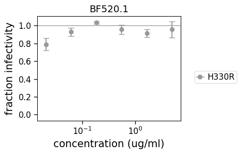
Fitting some problematic curves
Here we demonstrate that the method can also fit a problematic HIV curve that never reaches the IC50.
Data frame with data for virus not neutralized at any concentration:
[32]:
hiv_neut_data = pd.concat(
    [
        pd.DataFrame(
            {
                "serum": "BF520.1",
                "virus": "H330R",
                "replicate": 1,
                "concentration": [
                    0.020576132,
                    0.061728395,
                    0.185185185,
                    0.555555556,
                    1.666666667,
                    5,
                ],
                "fraction infectivity": [
                    0.721440083,
                    0.882537173,
                    1.01964302,
                    0.904916836,
                    0.870465533,
                    0.866026089,
                ],
            }
        ),
        pd.DataFrame(
            {
                "serum": "BF520.1",
                "virus": "H330R",
                "replicate": 2,
                "concentration": [
                    0.020576132,
                    0.061728395,
                    0.185185185,
                    0.555555556,
                    1.666666667,
                    5,
                ],
                "fraction infectivity": [
                    0.857961054,
                    0.973908617,
                    1.04569174,
                    1.007668321,
                    0.959208349,
                    1.046646303,
                ],
            }
        ),
    ]
)
hiv_neut_data.head()
[32]:
| serum | virus | replicate | concentration | fraction infectivity | |
|---|---|---|---|---|---|
| 0 | BF520.1 | H330R | 1 | 0.0206 | 0.721 |
| 1 | BF520.1 | H330R | 1 | 0.0617 | 0.883 |
| 2 | BF520.1 | H330R | 1 | 0.185 | 1.02 |
| 3 | BF520.1 | H330R | 1 | 0.556 | 0.905 |
| 4 | BF520.1 | H330R | 1 | 1.67 | 0.87 |
Fit and plot curve:
[33]:
hiv_fit = neutcurve.CurveFits(hiv_neut_data)
_ = hiv_fit.plotSera(xlabel="concentration (ug/ml)")
[34]:
hiv_fit.fitParams()
[34]:
| serum | virus | replicate | nreplicates | ic50 | ic50_bound | ic50_str | midpoint | midpoint_bound | midpoint_bound_type | slope | top | bottom | r2 | rmsd | |
|---|---|---|---|---|---|---|---|---|---|---|---|---|---|---|---|
| 0 | BF520.1 | H330R | average | 2 | 5 | lower | >5 | 1.63e+04 | 5 | lower | 3.56 | 1 | 0 | -0.932 | 0.101 |
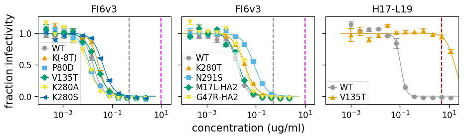
Drawing vertical lines
It can sometimes be useful to draw vertical lines on the plot, such as to indicate concentrations used for selection experiments. This can be done in a highly customized way using the option to neutcurve.curvefits.CurveFits.plotSera() as in the example below:
[35]:
fig, axes = fits.plotSera(
    max_viruses_per_subplot=6,
    nrow=1,
    ncol=None,
    xlabel="concentration (ug/ml)",
    vlines={
        "FI6v3": [{"x": 0.5}, {"x": 10, "color": "magenta"}],
        "H17-L19": [{"x": 5, "linestyle": "--", "color": "red"}],
    },
)
Additional plot customization
The plots are returned as figures / axes, so can be customized just like any other generated plot. For instance, to customize axis ticks and labels, you can do the below:
[36]:
fig2, axes2 = fits.plotSera(
    max_viruses_per_subplot=6,
    nrow=1,
    ncol=None,
    xlabel="log10 concentration (ug/ml)",
    vlines={
        "FI6v3": [{"x": 0.5}, {"x": 10, "color": "magenta"}],
        "H17-L19": [{"x": 5, "linestyle": "--", "color": "red"}],
    },
)
_ = axes2.ravel()[-1].set_xticks([1e-3, 1e-2, 1e-1, 1, 10])
_ = axes2.ravel()[-1].set_xticklabels(["-3", "-2", "-1", "0", "1"])
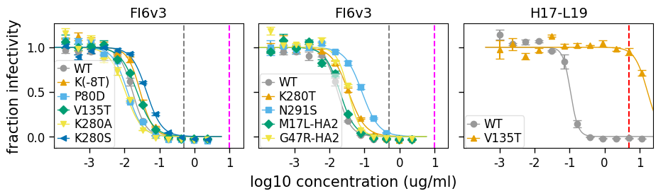
This assumes the plotting was done using sharex=True and sharey=True (on by default), which makes all axes share the same x-ticks so they can be set for just the last plot. Otherwise you need to set the ticks for each axis separately.