Hill-curve neutralization

Mathematical form of curves

The neutralization curve is fit to measurements of the fraction infectivity remaining \(f\left(c\right)\) at several different serum concentrations \(c\). The equation for the curve is:

\[f(c) = b + \frac{t - b}{1 + (c/m)^s}\]

where \(m\) is the midpoint of the curve, \(t\) is the “top” of the curve, \(b\) is the bottom of the curve, and \(s\) is the “slope” or Hill coefficient of the curve.

If the curve spans from completely non-neutralized (100% infectivity remaining) to completely neutralized (0% infectivity remaining), then \(t = 1\) and \(b = 0\). In this case, Equation (1) is identical to 1 minus the Hill equation defined on Wikipedia.

However, it will not always be the case that the top and bottom are at 1 and 0. The reason is that some antibodies and sera do not go to complete neutralization (see here for a discussion of the phenomenon for HIV). For such antibodies, \(b\) will in general be \(>0\). Therefore, in the fitting you have the option of constraining the top and bottom to \(t = 1\) and \(b = 0\), or to fit them as free parameters. The default is to constrain the top to \(t = 1\) and the bottom to \(b = 0\), but you should look at your curves to ensure this makes sense–and if they don’t plateau at complete neutralization, set the bottom \(b\) to be a free parameter to allow for incomplete neutralization.

Since \(f\left(c\right)\) in Equation (1) is the fraction infectivity, we expect \(f\left(c\right)\) to get smaller as the antibody concentration increases. Just be aware that some papers will plot fraction neutralized rather than fraction infectivity; fraction neutralized is \(1 - f\left(c\right)\). If your data is fraction neutralized, you should convert it to fraction infectivity before using this package, or use the option described in the docs for neutcurve.hillcurve.HillCurve.

Fitting using the HillCurve class

The curves are fit using the neutcurve.hillcurve.HillCurve class. For fitting to actual data, you will typically want to fit these curves via neutcurve.curvefits.CurveFits as described in Fitting curves to real data, particularly when there are multiple samples being fit at once. Nonetheless, here we illustrate the basic fitting to a single sample using neutcurve.hillcurve.HillCurve.

First, we import the requisite Python modules:

import pandas as pd

import neutcurve

Set pandas display options:

pd.set_option("display.float_format", "{:.5f}".format)

Now we get example data to plot. We use as our example the neutralization of wildtype (WT) A/WSN/1933 (H1N1) influenza by the broadly neutralizing antibody FI6v3 as determined in Fig 6a of Doud et al (2018). The numerical data in that figure in tidy form are available in a CSV file. We read the data and get just the measurements for replicate 1 of the wildtype virus against FI6v3:

fi6v3_datafile = "Doud_et_al_2018-neutdata.csv"

data = (
    pd.read_csv(fi6v3_datafile)
    .query('(serum == "FI6v3") & (virus == "WT") & (replicate == 1)')[
        ["concentration", "fraction infectivity"]
    ]
    .reset_index(drop=True)
)
data.round(5)

	concentration	fraction infectivity
0	0.00020	1.01373
1	0.00048	0.94201
2	0.00112	0.99285
3	0.00260	0.96621
4	0.00607	0.95670
5	0.01417	0.58633
6	0.03305	0.16945
7	0.07712	0.01413
8	0.17995	-0.02539
9	0.41989	-0.03255
10	0.97974	-0.03667
11	2.28606	-0.02877

As can be seen above, the data give the fraction activity at each antibody concentration (which in this case is in \(\mu\)g/ml).

Now we initialize a neutcurve.hillcurve.HillCurve with these data:

curve = neutcurve.HillCurve(data["concentration"], data["fraction infectivity"])

We can now look at the values of each of the four fit parameters that define the curve:

print(
    f"The top (t) is {curve.top:.3g}\n"
    f"The bottom (b) is {curve.bottom:.3g}\n"
    f"The midpoint (m) is {curve.midpoint:.3g}\n"
    f"The slope (Hill coefficient)s is {curve.slope:.3g}"
)

The top (t) is 1
The bottom (b) is 0
The midpoint (m) is 0.0167
The slope (Hill coefficient)s is 2.5

Note that the top and bottom are one and zero as they were constrained to those values. If you want to change whether the top and/or bottom are fixed or fit, you can do that using the and arguments to neutcurve.hillcurve.HillCurve as described in the docs for that class. For instance, below we fit the top and fix the bottom (it makes very little difference for this particular dataset):

curve2 = neutcurve.HillCurve(
    data["concentration"], data["fraction infectivity"], fixtop=False
)

print(
    f"The top (t) is {curve2.top:.3g}\n"
    f"The bottom (b) is {curve2.bottom:.3g}\n"
    f"The midpoint (m) is {curve2.midpoint:.3g}\n"
    f"The slope (Hill coefficient)s is {curve2.slope:.3g}"
)

The top (t) is 0.987
The bottom (b) is 0
The midpoint (m) is 0.0169
The slope (Hill coefficient)s is 2.57

We can also get the IC50, which is the concentration where \(f\left(c\right) = 0.5\). The IC50 will be equal to the midpoint \(m\) when the top (\(t\)) is one and the bottom (\(b\)) is zero, but otherwise it may be different than the IC50. For this particular dataset, the IC50 is very close to the midpoint:

print(f"The IC50 is {curve.ic50():.3g}")

The IC50 is 0.0167

Note that neutcurve.hillcurve.HillCurve.ic50() has a option for how to handle computing the IC50 if it doesn’t fall within the range of the provided concentrations and so cannot be interpolated (see the docs for that method for details). This doesn’t matter for this particular dataset, however, since the IC50 falls within the range of the data. There are also two other methods that deal with IC50s that cannot be interpolated and so are only determinable as upper / lower bounds:

• neutcurve.hillcurve.HillCurve.ic50_bound()

• neutcurve.hillcurve.HillCurve.ic50_str()

print(curve.ic50_bound())
print(curve.ic50_str())

interpolated
0.0167

We can generalize the IC50 using neutcurve.hillcurve.HillCurve.icXX(), which will compute the concentration at which an arbitrary fraction of virus is expected to be neutralized (note that this is fraction neutralized, which is one minus the fraction infectivity). For instance:

print(f"The IC95 is {curve.icXX(0.95):.3g}")

The IC95 is 0.0541

Note that neutcurve.hillcurve.HillCurve.icXX() has a argument that determines how we handle the case when the ICXX is outside of the range of measured concentrations, and that there are two other methods that deal with ICXXs that cannot be interpolated and are only determinable as upper / lower bounds:

• neutcurve.hillcurve.HillCurve.icXX_bound()

• neutcurve.hillcurve.HillCurve.icXX_str()

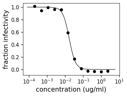
We can plot the neutralization curve using the neutcurve.hillcurve.HillCurve.plot() function. This returns a matplotlib figure and axis instance:

fig, ax = curve.plot(xlabel="concentration (ug/ml)")

If you want to save the figure, do this using its savefig method, possibly calling tight_layout command first if there is clipping.

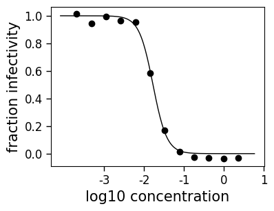
If you want to adjust the x-axis tick locations / labels, you can do it on the ax object returned as part of the plot:

fig2, ax2 = curve.plot(xlabel="concentration (ug/ml)")
_ = ax2.set_xticks([1e-3, 1e-2, 1e-1, 1, 10])
_ = ax2.set_xticklabels(["-3", "-2", "-1", "0", "1"])
_ = ax2.set_xlabel("log10 concentration")

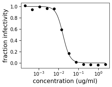
You can also plot the curve only in the bounds of the data using the draw_in_bounds=True option:

fig, ax = curve.plot(xlabel="concentration (ug/ml)", draw_in_bounds=True)

Quantifying goodness of fit

We can quantify the goodness of fit by the coefficient of determination (\(R^2\)) using HillCurve.r2, which will be one if the curve perfectly fits the data and less than one otherwise. Essentially, this corresponds to the fraction of the variation in the data explained by the curve. A value of <0 means the fit is worse than just drawing a straight line through the data:

round(curve.r2, 3)

0.996

We can also quantify how well each data point is fit on average with the root mean square deviation (the square root of the mean residual) A value of zero means the curve perfectly fits the data. This is returned by HillCurve.rmsd:

round(curve.rmsd, 3)

0.028

In general, you might consider a curve fit to be “good” if either the r2 is close to one, or the rmsd is close to zero. Usually they will be correlated, but if the data essentially fall on a flat line (no or complete neutralization at all tested concentrations), then you could have a poor r2 close to zero but still a small rmsd because in this case the curve would fit the data well (small rmsd) but would not be much better than a line (so poor r2) simply because the data are basically linear.