Fit model to data
We will fit a Polyclonal model to the RBD antibody mix we simulated.
First, we read in that simulated data. Recall that we simulated both “exact” and “noisy” data, with several average per-library mutations rates, and at six different concentrations. Here we analyze the noisy data for the library with an average of 3 mutations per gene, measured at three different concentrations, as this represents a fairly realistic representation of a real experiment:
[1]:
import requests
import tempfile

import pandas as pd

import polyclonal

noisy_data = (
    pd.read_csv("RBD_variants_escape_noisy.csv", na_filter=None)
    .query('library == "avg3muts"')
    .query("concentration in [0.25, 1, 4]")
    .reset_index(drop=True)
)

noisy_data
[1]:
| library | barcode | concentration | prob_escape | aa_substitutions | IC90 | |
|---|---|---|---|---|---|---|
| 0 | avg3muts | AAAACTGCTGAGGAGA | 0.25 | 0.054700 | 0.08212 | |
| 1 | avg3muts | AAAAGCAGGCTACTCT | 0.25 | 0.000000 | 0.08212 | |
| 2 | avg3muts | AAAAGCTATAGGTGCC | 0.25 | 0.007613 | 0.08212 | |
| 3 | avg3muts | AAAAGGTATTAGTGGC | 0.25 | 0.001363 | 0.08212 | |
| 4 | avg3muts | AAAAGTGCCTTCGTTA | 0.25 | 0.000000 | 0.08212 | |
| ... | ... | ... | ... | ... | ... | ... |
| 119995 | avg3muts | GAGCATGATCGACGAA | 1.00 | 0.000000 | Y508V H519I | 0.10830 |
| 119996 | avg3muts | GAGCATGATCGACGAA | 4.00 | 0.000000 | Y508V H519I | 0.10830 |
| 119997 | avg3muts | CTTAAAATAGCTGGTC | 0.25 | 0.000000 | Y508W | 0.08212 |
| 119998 | avg3muts | CTTAAAATAGCTGGTC | 1.00 | 0.012260 | Y508W | 0.08212 |
| 119999 | avg3muts | CTTAAAATAGCTGGTC | 4.00 | 0.000000 | Y508W | 0.08212 |
120000 rows × 6 columns
For spatial regularization (encouraging epitopes to be structurall proximal residues), we read the inter-residue distances in angstroms from PDB 6m0j:
[2]:
# we read the PDB from the webpage into a temporary file and get the distances from that.
# you could also just download the file manually and then read from it.
r = requests.get("https://files.rcsb.org/download/6XM4.pdb")
with tempfile.NamedTemporaryFile() as tmpf:
    _ = tmpf.write(r.content)
    tmpf.flush()
    spatial_distances = polyclonal.pdb_utils.inter_residue_distances(tmpf.name, ["A"])

spatial_distances
[2]:
| site_1 | site_2 | distance | chain_1 | chain_2 | |
|---|---|---|---|---|---|
| 0 | 27 | 28 | 1.332629 | A | A |
| 1 | 27 | 29 | 4.612508 | A | A |
| 2 | 27 | 30 | 8.219518 | A | A |
| 3 | 27 | 31 | 11.016782 | A | A |
| 4 | 27 | 32 | 13.087037 | A | A |
| ... | ... | ... | ... | ... | ... |
| 548623 | 1308 | 1310 | 30.826773 | A | A |
| 548624 | 1308 | 1311 | 75.350853 | A | A |
| 548625 | 1309 | 1310 | 12.374796 | A | A |
| 548626 | 1309 | 1311 | 115.681534 | A | A |
| 548627 | 1310 | 1311 | 106.112328 | A | A |
548628 rows × 5 columns
Initialize a Polyclonal model with these data, including three epitopes. We know from prior work the three most important epitopes and a key mutation in each, so we use this prior knowledge to “seed” initial guesses that assign large escape values to a key site in each epitope:
site 417 for class 1 epitope, which is often the least important
site 484 for class 2 epitope, which is often the dominant one
site 444 for class 3 epitope, which is often the second most dominant one
[3]:
poly_abs = polyclonal.Polyclonal(
    data_to_fit=noisy_data,
    activity_wt_df=pd.DataFrame.from_records(
        [
            ("1", 1.0),
            ("2", 3.0),
            ("3", 2.0),
        ],
        columns=["epitope", "activity"],
    ),
    site_escape_df=pd.DataFrame.from_records(
        [
            ("1", 417, 10.0),
            ("2", 484, 10.0),
            ("3", 444, 10.0),
        ],
        columns=["epitope", "site", "escape"],
    ),
    data_mut_escape_overlap="fill_to_data",
    spatial_distances=spatial_distances,
)
Now fit the Polyclonal model, logging output every 100 steps. Note how the fitting first just fits a site level model to estimate the average effects of mutations at each site, and then fits the full model. Here we fix the Hill coefficient at one and the non-neutralized fraction at zero:
[4]:
# NBVAL_IGNORE_OUTPUT
opt_res = poly_abs.fit(
    logfreq=200,
    reg_escape_weight=0.01,
    reg_spatial2_weight=1e-5,
    reg_uniqueness2_weight=0,
    fix_non_neutralized_frac=True,
    fix_hill_coefficient=True,
)
#
# Fitting site-level model.
# Starting optimization of 522 parameters at Tue Apr  4 16:01:08 2023.
        step    time_sec        loss    fit_loss  reg_escape  reg_spread reg_spatial reg_uniqueness reg_uniqueness2 reg_activity reg_hill_coefficient reg_non_neutralized_frac
           0     0.10483      2991.9      2980.2     0.29701           0           0              0               0       11.418                    0                        0
         200      24.563        1876      1836.9      2.3802           0      25.111              0               0       11.569                    0                        0
         308      37.745      1873.6      1835.4      2.3448           0      24.241              0               0       11.592                    0                        0
# Successfully finished at Tue Apr  4 16:01:45 2023.
#
# Fitting model.
# Starting optimization of 5799 parameters at Tue Apr  4 16:01:45 2023.
        step    time_sec        loss    fit_loss  reg_escape  reg_spread reg_spatial reg_uniqueness reg_uniqueness2 reg_activity reg_hill_coefficient reg_non_neutralized_frac
           0     0.13785      2026.1      1960.5      29.725  3.6371e-30      24.241              0               0       11.592                    0                        0
         200      31.743      492.84      378.86      33.574      20.624      46.484              0               0         13.3                    0                        0
         400      62.818      479.16       366.6      32.471      21.461      45.134              0               0       13.489                    0                        0
         600      93.955      476.55      364.79      31.686      22.005      44.596              0               0       13.467                    0                        0
         800      124.81      469.69      358.68      31.313      22.319      43.888              0               0       13.489                    0                        0
        1000      155.41      466.36      356.22      31.011      22.471      43.178              0               0       13.479                    0                        0
        1200      186.12      462.73      353.63      30.727      22.423      42.489              0               0       13.454                    0                        0
        1400      216.23      462.18      352.96      30.669      22.483      42.602              0               0       13.464                    0                        0
        1600      246.06      457.12      347.99      30.439      22.776      42.496              0               0       13.421                    0                        0
        1800      275.75      456.23      347.31      30.348      22.746      42.382              0               0       13.447                    0                        0
        1826      279.48      456.23      347.31      30.345       22.75      42.375              0               0       13.449                    0                        0
# Successfully finished at Tue Apr  4 16:06:25 2023.
We can now visualize the resulting curve fits and activity values and compare them to the “true” activity values used to simulate the data. Note that the Hill coefficients are one and the non-neutralized fractions are zero because we fixed them as such above:
[5]:
poly_abs.curve_specs_df.round(1)
[5]:
| epitope | activity | hill_coefficient | non_neutralized_frac | |
|---|---|---|---|---|
| 0 | 1 | 1.5 | 1.0 | 0.0 |
| 1 | 2 | 3.2 | 1.0 | 0.0 |
| 2 | 3 | 2.4 | 1.0 | 0.0 |
[6]:
# NBVAL_IGNORE_OUTPUT
poly_abs.curves_plot()
[6]:
[7]:
# NBVAL_IGNORE_OUTPUT
poly_abs.activity_wt_barplot()
[7]:
[8]:
# NBVAL_IGNORE_OUTPUT

import altair as alt

true_activities = pd.read_csv("RBD_activity_wt_df.csv")


activity_wt_comparison = (
    pd.concat(
        [
            poly_abs.activity_wt_df.rename(columns={"activity": "predicted"}),
            true_activities.rename(columns={"activity": "actual"}).drop(
                columns="epitope"
            ),
        ],
        axis=1,
    )
).melt(
    id_vars=["epitope"],
    value_vars=["actual", "predicted"],
    var_name="value_type",
    value_name="wildtype activity",
)

alt.Chart(activity_wt_comparison).mark_bar(size=35).encode(
    x="value_type:O",
    y="wildtype activity:Q",
    color=alt.Color(
        "epitope:N", scale=alt.Scale(range=list(poly_abs.epitope_colors.values()))
    ),
    column="epitope:N",
    tooltip=["value_type", alt.Tooltip("wildtype activity", format=".3f"), "epitope"],
).properties(width=100, height=125)
[8]:
Similarly, we can visualize the resulting fits for the escape values, and compare them to the “true” escape values used to simulate the data. Note how entries can be filtered by how many variants a mutation is seen in (times_seen):
[9]:
# NBVAL_IGNORE_OUTPUT
poly_abs.mut_escape_plot()
[9]:
For these simulated data, we can also see how well the fit model does on the “true” simulated values from a library with a different (higher) mutation rate. We therefore read in the “exact” simulated data from a library with a different mutation rate:
[10]:
exact_data = (
    pd.read_csv("RBD_variants_escape_exact.csv", na_filter=None)
    .query('library == "avg3muts"')
    .query("concentration in [0.25, 1, 0.5]")
    .reset_index(drop=True)
)
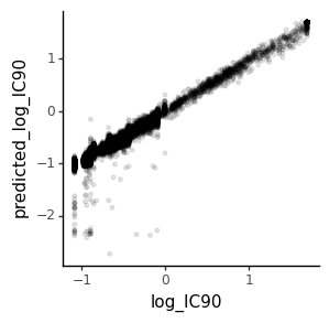
We will compare the true simulated IC90 values to those predicted by the fit model. We make the comparison on a log scale, and clip IC90s at values >50 as likely to be way outside the dynamic range given the concentrations used:
[11]:
# NBVAL_IGNORE_OUTPUT

import numpy

from plotnine import *

max_ic90 = 50

# we only need the variants, not the concentration for the IC90 comparison
ic90s = (
    exact_data[["aa_substitutions", "IC90"]]
    .assign(IC90=lambda x: x["IC90"].clip(upper=max_ic90))
    .drop_duplicates()
)

ic90s = poly_abs.icXX(ic90s, x=0.9, col="predicted_IC90", max_c=max_ic90)

ic90s = ic90s.assign(
    log_IC90=lambda x: numpy.log10(x["IC90"]),
    predicted_log_IC90=lambda x: numpy.log10(x["predicted_IC90"]),
)

corr = ic90s["log_IC90"].corr(ic90s["predicted_log_IC90"]) ** 2
print(f"Correlation (R^2) is {corr:.2f}")

ic90_corr_plot = (
    ggplot(ic90s)
    + aes("log_IC90", "predicted_log_IC90")
    + geom_point(alpha=0.1, size=1)
    + theme_classic()
    + theme(figure_size=(3, 3))
)

_ = ic90_corr_plot.draw()
# ic90_corr_plot.save('IC90_pred_vs_actual.pdf', height=3.5, width=3.5)
Correlation (R^2) is 0.97
Next we see how well the model predicts the variant-level escape probabilities \(p_v\left(c\right)\), by reading in exact data from the simulations, and then making predictions of escape probabilities. We both examine and plot the correlations:
[12]:
# NBVAL_IGNORE_OUTPUT

exact_vs_pred = poly_abs.prob_escape(variants_df=exact_data)

print(f"Correlations (R^2) at each concentration:")
display(
    exact_vs_pred.groupby("concentration")
    .apply(lambda x: x["prob_escape"].corr(x["predicted_prob_escape"]) ** 2)
    .rename("correlation (R^2)")
    .reset_index()
    .round(2)
)

pv_corr_plot = (
    ggplot(exact_vs_pred)
    + aes("prob_escape", "predicted_prob_escape")
    + geom_point(alpha=0.1, size=1)
    + facet_wrap("~ concentration", nrow=1)
    + theme_classic()
    + theme(figure_size=(3 * exact_vs_pred["concentration"].nunique(), 3))
)

_ = pv_corr_plot.draw()
Correlations (R^2) at each concentration:
| concentration | correlation (R^2) | |
|---|---|---|
| 0 | 0.25 | 0.99 |
| 1 | 0.50 | 1.00 |
| 2 | 1.00 | 1.00 |
We also examine the correlation between the “true” and inferred mutation-escape values, \(\beta_{m,e}\). In general, it’s necessary to ensure the epitopes match up for this type of comparison as it is arbitrary which epitope in the model is given which name. But above we seeded the epitopes at the site level using site_effects_df when we initialized the Polyclonal object, so they match up with class 1, 2, and 3:
[13]:
# NBVAL_IGNORE_OUTPUT

import altair as alt

mut_escape_pred = pd.read_csv("RBD_mut_escape_df.csv").merge(
    (
        poly_abs.mut_escape_df.assign(
            epitope=lambda x: "class " + x["epitope"].astype(str)
        ).rename(columns={"escape": "predicted escape"})
    ),
    on=["mutation", "epitope"],
    validate="one_to_one",
)

print("Correlation (R^2) between predicted and true values:")
corr = (
    mut_escape_pred.groupby("epitope")
    .apply(lambda x: x["escape"].corr(x["predicted escape"]) ** 2)
    .rename("correlation (R^2)")
    .reset_index()
)
display(corr.round(2))

# for testing since we nbval ignore cell output
assert (
    numpy.allclose(
        corr["correlation (R^2)"], numpy.array([0.60, 0.96, 0.95]), atol=0.02
    )
    == True
)

corr_chart = (
    alt.Chart(mut_escape_pred)
    .encode(
        x="escape",
        y="predicted escape",
        color=alt.Color(
            "epitope", scale=alt.Scale(range=list(poly_abs.epitope_colors.values()))
        ),
        tooltip=["mutation", "epitope"],
    )
    .mark_point(opacity=0.5)
    .properties(width=250, height=250)
    .facet(column="epitope")
    .resolve_scale(
        x="independent",
        y="independent",
    )
)

corr_chart
Correlation (R^2) between predicted and true values:
| epitope | correlation (R^2) | |
|---|---|---|
| 0 | class 1 | 0.60 |
| 1 | class 2 | 0.96 |
| 2 | class 3 | 0.95 |
[13]:
The correlations are strongest for the dominant epitope (class 2), which makes sense as this will drive the highest escape signal.