bottlenecks

Estimation of bottlenecks during experiments.

dms_variants.bottlenecks.estimateBottleneck(df, *, n_pre_col='n_pre', n_post_col='n_post', pseudocount=0.5, min_variants=100)

Estimate neutral bottleneck from pre- and post-selection counts.

This function estimates a bottleneck between a pre- and post-selection condition based on changes in frequencies of variants that are all selectively neutral with respect to each other. So in a deep mutational scanning experiment, you could apply it to a data frame of pre- and post- selection counts for all wildtype variants (or all synonymous variants if you assume those are neutral). Do not include variants that are expected to have different “fitness” values.

The inference of the bottleneck size appears fairly accurate if the following conditions are met:

1. The sequencing depth substantially exceeds the actual bottleneck size, so that differences in pre- and post-selection frequencies are the result of the bottleneck rather than sampling errors in the counts.

2. There are a reasonably large number of variants.

3. The variants are all of the same fitness (so to emphasize, only apply to wildtype (and possibly synonymous) variants in your experiment.

The bottleneck is estimated using the method described in Equation (8) of Ghafari et al (2020). Specifically, let the pre- and post-selection frequencies of each variant \(v = 1, \ldots, V\) be \(f_v^{\rm{pre}}\) and \(f_v^{\rm{post}}\). (These frequencies are estimated from the counts plus a pseudocount). Then the log likelihood of a bottleneck of size \(N\) is estimated as

\[\mathcal{L}\left(N\right) = \sum_{v=1}^V \ln \mathcal{N}\left(f_v^{\rm{post}}; f_v^{\rm{pre}}, \frac{f_v^{\rm{pre}}\left(1 - f_v^{\rm{pre}}\right)}{N}\right)\]

where \(\mathcal{N}\left(x; \mu, \sigma^2\right)\) is the probability density function of a normal distribution with mean \(\mu\) and variance \(\sigma^2\).

Note that the returned value is the per-variant bottleneck (the total bottleneck \(N\) divided by the number of variants \(V\)). The reason we return the bottleneck per-variant is that you may have subsetted on just some variants (i.e., wildtype ones) to estimate the bottleneck.

Parameters:

• df (pandas.DataFrame) – Data frame with counts. Each row gives counts for a different variant.

• n_pre_col (str) – Column in df with pre-selection counts.

• n_post_col (str) – Column in df with post-selection counts.

• pseudocount (float') – Pseudocount added to counts to estimate frequencies.

• min_variants (int) – The inference will not be reliable if there are too few variants in df. Raise an error if fewer than this many variants.

Returns:

The estimated bottleneck per variant, which is the mean number of copies of each variant that survives the bottleneck.

Return type:

float

Example

Here is an example testing the bottleneck inferences on simulated data. Plausible data are simulated under a range of bottlenecks, and then the bottleneck size is estimated with estimateBottleneck(). As can be seen below, the estimated bottleneck is within 10% of the real one for bottleneck sizes ranging from half the number of variants to 10X the number of variants. The estimates only start to break down when the bottleneck size becomes so large it is comparable to the overall sequencing depth, so that the bottleneck is no longer the main source of noise. In addition, plots are shown at the bottom of the example of the counts distribution in each simulation.

>>> import matplotlib.pyplot as plt
>>> import numpy
>>> import pandas as pd
>>> from dms_variants.bottlenecks import estimateBottleneck

>>> numpy.random.seed(1)  # seed for reproducible output

>>> nvariants = 100000  # number of variants in library
>>> depth = nvariants * 100  # sequencing depth 100X library size

Initial counts are multinomial draw from Dirichlet-distributed freqs:

>>> freqs_pre = numpy.random.dirichlet(numpy.full(nvariants, 2))
>>> n_pre = numpy.random.multinomial(depth, freqs_pre)

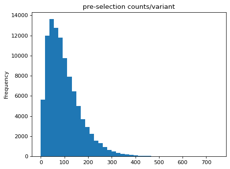
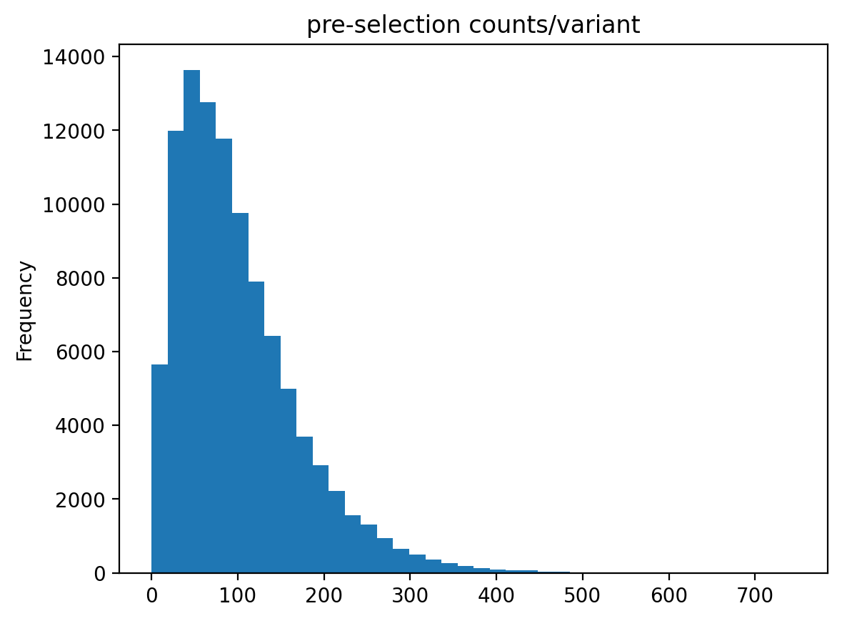
Create data frame with pre-selection counts and plot distribution:

>>> df = pd.DataFrame({'n_pre': n_pre})
>>> _ = df['n_pre'].plot.hist(bins=40,
...                           title='pre-selection counts/variant')

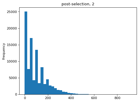
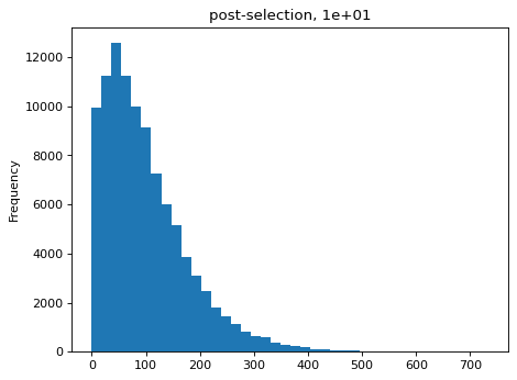
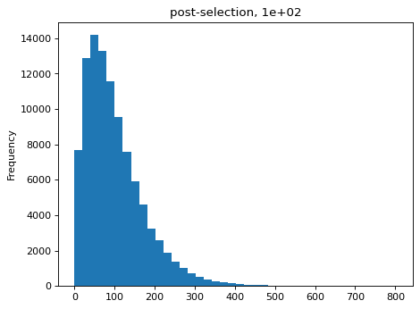
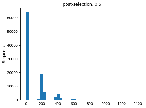
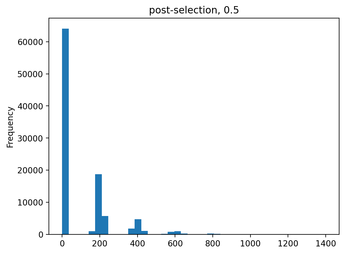
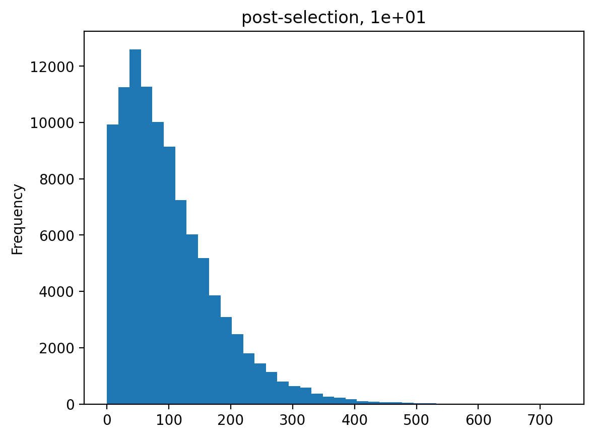
Simulate counts after bottlenecks of various sizes, simulated as re-normalized multinomial draws of bottleneck size used to to parameterize new multinomial draws of sequencing counts. Then estimate the bottlenecks on the simulated data and compare to actual value:

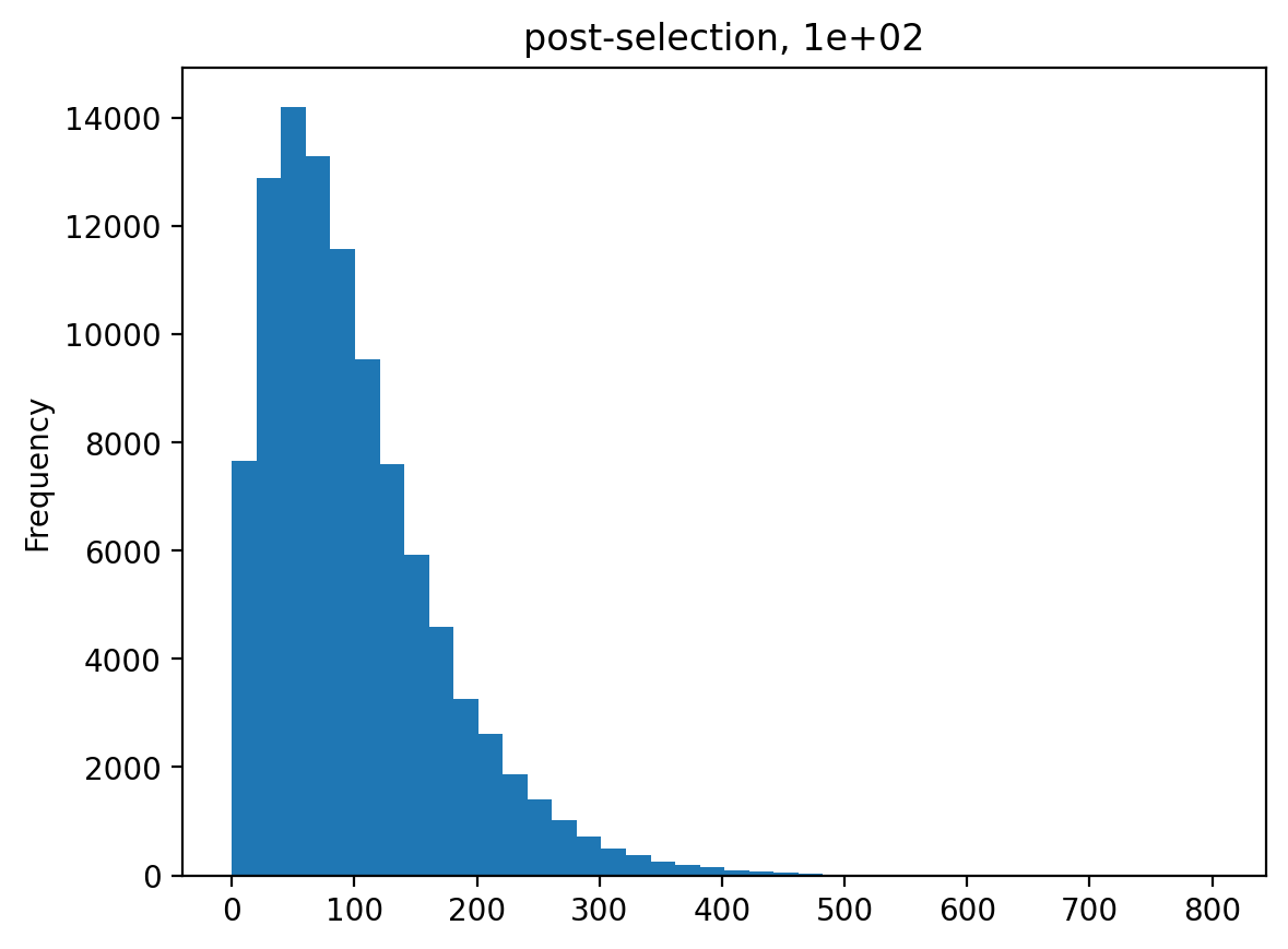
>>> estimates = []
>>> for n_per_variant in [0.5, 2, 10, 100]:
...     n_bottle = numpy.random.multinomial(
...                                    int(n_per_variant * nvariants),
...                                    n_pre / n_pre.sum())
...     freqs_bottle = n_bottle / n_bottle.sum()
...     n_post = numpy.random.multinomial(depth, freqs_bottle)
...     df['n_post'] = n_post
...     _ = plt.figure()
...     _ = df['n_post'].plot.hist(
...                       bins=40,
...                       title=f"post-selection, {n_per_variant:.1g}")
...     n_per_variant_est = estimateBottleneck(df)
...     estimates.append((n_per_variant, n_per_variant_est))
>>> estimates_df = pd.DataFrame.from_records(
...                                 estimates,
...                                 columns=['actual', 'estimated'])
>>> estimates_df  
   actual  estimated
0     0.5        0.5
1     2.0        2.0
2    10.0        9.3
3   100.0       50.4

Confirm that estimates are good when bottleneck is small:

>>> numpy.allclose(
...         estimates_df.query('actual <= 10')['actual'],
...         estimates_df.query('actual <= 10')['estimated'],
...         rtol=0.1)
True

(png, hires.png, pdf)

(png, hires.png, pdf)

(png, hires.png, pdf)

(png, hires.png, pdf)

(png, hires.png, pdf)