hillcurve

Defines HillCurve for fitting neutralization curves.

class neutcurve.hillcurve.HillCurve(cs, fs, *, infectivity_or_neutralized='infectivity', fix_slope_first=True, fs_stderr=None, fixbottom=0, fixtop=1, fixslope=False, fitlogc=False, use_stderr_for_fit=False, init_slope=1.5, no_curve_fit_first=False)

Bases: object

A fitted Hill curve, optionally with free baselines.

Fits \(f\left(c\right) = b + \frac{t - b}{1 + \left(c/m\right)^s}\) where \(f\left(c\right)\) is the fraction infectivity remaining at concentration \(c\), \(m\) is the midpoint of the neutralization curve, \(t\) is the top value (e.g., 1), \(b\) is the bottom value (e.g., 0), and \(s\) is the slope of the curve. Because \(f\left(c\right)\) is the fraction infectivity remaining, we expect \(f\left(c\right)\) to get smaller as \(c\) gets larger. This should lead us to fit \(s > 0\).

When \(t = 1\) and \(b = 0\), this equation is identical to the Hill curve, except that we are calculating the fraction unbound rather than the fraction bound.

You may want to fit the fraction neutralized rather than the fraction infectivity. In that case, set infectivity_or_neutralized=’neutralized’ and then the equation that is fit will be :math:`fleft(cright) = t + frac{b - t}{1 + left(c/mright)^s}, which means that fleft(cright) gets larger rather than smaller as \(c\) increases.

Args:

cs (array-like)

Concentrations of antibody / serum.

fs (array-like)

Fraction infectivity remaining at each concentration.

infectivity_or_neutralized ({‘infectivity’, ‘neutralized’})

Fit the fraction infectivity (\(f\left(c\right)\) decreases as \(c\) increases) or neutralized (\(f\left(c\right)\) increases as \(c\) increases). See equations above.

fix_slope_first (bool)

If True, initially fit with fixed slope, and then start from those values to re-fit all parameters including slope.

fs_stderr (None or array-like)

If not None, standard errors on fs.

fixbottom (False, float, or tuple/list of length 2)

If False, fit bottom of curves as free parameter. If float, fix bottom of curve to that value. If length-2 array, constrain bottom to be in that range.

fixtop (False, float, or tuple/list of length 2)

If False, fit top of curves as free parameter. If float, fix top of curve to that value. If length-2 array, constrain top to be in that range.

fixslope (False, float, or tuple/list of length 2)

If False, fit slope of curves as free parameter. If float, fix slope to that value. If length-2 array, constrain slope to be in that range.

fitlogc (bool)

Do we do the actual fitting on the concentrations or log concentrations? Gives equivalent results in principle, but fitting to log concentrations may be more efficient in pratice.

use_stderr_for_fit (bool)

Do we use fs_stderr for the fitting, or just for plotting? Usually it is a good idea to set to False and not use for fitting if you only have a few replicates, and the standard error is often not that accurate and so will weight some points much more than others in a way that may not be justified.

init_slope (float)

Initial value of slope used in fitting. If fixslope is set to a single value, it overrides this parameter. If fixslope is set to a range, init_slope is adjusted up/down to be in that range.

no_curve_fit_first (bool)

Normally the method first tries to do the optimization with curve_fit from scipy, and if that fails then tries scipy.optimize.minimize. If you set this to True, it skips trying with curve_fit. In general, this option is for debugging by knowledgeable developers, and you should not be using it otherwise.

Attributes:

cs (numpy array)

Concentrations, sorted from low to high.

fs (numpy array)

Fraction infectivity, ordered to match sorted concentrations.

fs_stderr (numpy array or None)

Standard errors on fs.

bottom (float)

Bottom of curve, \(b\) in equation above.

top (float)

Top of curve, \(t\) in equation above.

midpoint (float)

Midpoint of curve, \(m\) in equation above. Note that the midpoint may not be the same as the ic50() if \(t \ne 1\) or \(b \ne 0\).

midpoint_bound (float)

Midpoint if it falls within fitted concentrations, otherwise the lowest concentration if below that or upper of above it.

midpoint_bound_type (str)

Is midpoint ‘interpolated’, or an ‘upper’ or ‘lower’ bound.

slope (float)

Hill slope of curve, \(s\) in equation above.

r2 (float)

Coefficient of determination indicating how well the curve fits the data (https://en.wikipedia.org/wiki/Coefficient_of_determination).

rmsd (float)

Root mean square deviation of fitted to actual values (square root of mean residual).

params_stdev (dict or None)

If standard deviations can be estimated on the fit parameters, keyed by ‘bottom’, ‘top’, ‘midpoint’, and ‘slope’ and gives standard erorr on each. Note if you have replicates we recommend fitting those separately and taking standard error rather than using fit stdev.

Use the ic50() method to get the fitted IC50. You can use ic50_stdev() to get the estimated standard deviation on the IC50, although if you have multiple replicates you may be better off just fitting to each separately and then taking standard error of the individual IC50s.

Here are some examples. First, we import the necessary modules:

>>> import numpy
>>>
>>> from neutcurve import HillCurve
>>> from neutcurve.colorschemes import CBPALETTE

Now simulate some data:

>>> m = 0.03
>>> s = 1.9
>>> b = 0.1
>>> t = 1.0
>>> cs = [0.002 * 2**x for x in range(9)]
>>> fs = [HillCurve.evaluate(c, m, s, b, t) for c in cs]

Now fit to these data, and confirm that the fitted values are close to the ones used for the simulation:

>>> neut = HillCurve(cs, fs, fixbottom=False)
>>> numpy.allclose(neut.midpoint, m, atol=1e-4)
True
>>> neut.midpoint_bound == neut.midpoint
True
>>> neut.midpoint_bound_type
'interpolated'
>>> numpy.allclose(neut.slope, s, atol=1e-3)
True
>>> numpy.allclose(neut.top, t, atol=1e-4)
True
>>> numpy.allclose(neut.bottom, b, atol=1e-3)
True
>>> for key, val in neut.params_stdev.items():
...     print(f"{key} = {val:.2g}")
midpoint = 0.062
slope = 6.3
top = 0
bottom = 0.73
>>> print(f"IC50: {neut.ic50():.3f} +/- {neut.ic50_stdev():.3f}")
IC50: 0.034 +/- 0.070

Since we fit the curve to simulated data where the bottom was 0.1 rather than 0, the midpoint and IC50 are different. Specifically, the IC50 is larger than the midpoint as you have to go past the midpoint to get down to 0.5 fraction infectivity:

>>> neut.ic50() > neut.midpoint
True
>>> numpy.allclose(neut.ic50(), 0.0337, atol=1e-4)
True
>>> numpy.allclose(0.5, neut.fracinfectivity(neut.ic50()))
True
>>> neut.fracinfectivity(neut.midpoint) > 0.5
True

Now here is an example where we constrain both the top and the bottom (to 1 and 0, respectively) and fit the curve. Now the midpoint and IC50 are the same:

>>> b2 = 0
>>> t2 = 1
>>> fs2 = [HillCurve.evaluate(c, m, s, b2, t2) for c in cs]
>>> neut2 = HillCurve(cs, fs2)
>>> numpy.allclose(neut2.midpoint, m)
True
>>> numpy.allclose(neut2.ic50(), m)
True

Now let’s fit to concentrations that are all less than the midpoint, so that we never get to complete neutralization. The estimated IC50 is unreliable, and so will be returned as None unless we call ic50() with method set to ‘bound’:

>>> cs3 = [1e-4 * 2**x for x in range(7)]
>>> (cs3[-1] < m)
True
>>> fs3 = [HillCurve.evaluate(c, m, s, b2, t2) for c in cs3]
>>> neut3 = HillCurve(cs3, fs3)
>>> neut3.ic50() is None
True
>>> numpy.allclose(neut3.ic50(method='bound'), cs3[-1])
True
>>> neut3.midpoint_bound == cs3[-1]
True
>>> neut3.midpoint_bound_type
'lower'

Note that we can determine if the IC50 is interpolated or an upper or lower bound using ic50_bound(), and get a nice string using ic50_str():

>>> neut.ic50_bound()
'interpolated'
>>> neut3.ic50_bound()
'lower'
>>> neut.ic50_str()
'0.0337'
>>> neut3.ic50_str()
'>0.0064'

We can use the dataframe() method to get the measured data and fit data at selected points. First, we do this just at measured points:

>>> neut.dataframe('measured').round(3)
   concentration  measurement    fit  stderr
0          0.002        0.995  0.995     NaN
1          0.004        0.981  0.981     NaN
2          0.008        0.932  0.932     NaN
3          0.016        0.791  0.791     NaN
4          0.032        0.522  0.522     NaN
5          0.064        0.272  0.272     NaN
6          0.128        0.154  0.154     NaN
7          0.256        0.115  0.115     NaN
8          0.512        0.104  0.104     NaN

Then we add in one more point:

>>> neut.dataframe([0.6]).round(3)
   concentration  measurement    fit  stderr
0          0.002        0.995  0.995     NaN
1          0.004        0.981  0.981     NaN
2          0.008        0.932  0.932     NaN
3          0.016        0.791  0.791     NaN
4          0.032        0.522  0.522     NaN
5          0.064        0.272  0.272     NaN
6          0.128        0.154  0.154     NaN
7          0.256        0.115  0.115     NaN
8          0.512        0.104  0.104     NaN
9          0.600          NaN  0.103     NaN

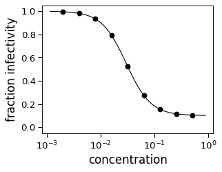
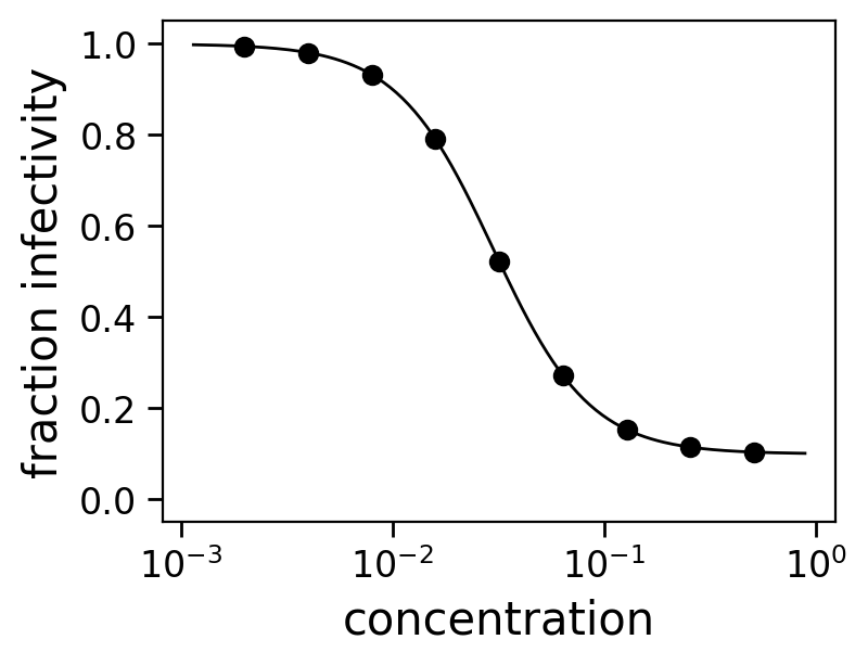
In reality, you’d typically just call dataframe() with the default argument of ‘auto’ to get a good range to plot. This is done if we call the HillCurve.plot() method:

>>> fig, ax = neut.plot()

(png, hires.png, pdf)

Finally, we confirm that we get the same result regardless of whether we fit using the concentrations in linear or log space:

>>> neut_linear = HillCurve(cs, fs, fitlogc=False, fixbottom=False)
>>> all(numpy.allclose(getattr(neut, attr), getattr(neut_linear, attr))
...     for attr in ['top', 'bottom', 'slope', 'midpoint'])
True

Demonstrate HillCurve.icXX():

>>> neut.icXX(0.95) is None
True
>>> neut.icXX_str(0.95)
'>0.512'
>>> neut.icXX_bound(0.95)
'lower'
>>> numpy.allclose(neut.icXX(0.95, method='bound'), neut.cs[-1])
True
>>> '{:.4f}'.format(neut.icXX(0.8), 4)
'0.0896'
>>> numpy.allclose(0.2, neut.fracinfectivity(neut.icXX(0.8)))
True

We can quantify the goodness of fit with HillCurve.r2. For these simulated data the fit is perfect (coefficient of determination of 1):

>>> round(neut.r2, 3)
1.0

We can also quantify the goodness of fit with HillCurve.rmsd: >>> round(neut.rmsd, 3) 0.0

Now fit with bounds on the parameters. First, we make bounds cover the true values:

>>> neut_bounds_cover = HillCurve(
...     cs, fs, fixbottom=(0, 0.2), fixtop=(0.9, 1), fixslope=(1, 2),
... )
>>> numpy.allclose(neut_bounds_cover.midpoint, m, atol=1e-4)
True
>>> numpy.allclose(neut_bounds_cover.slope, s, atol=1e-3)
True
>>> numpy.allclose(neut_bounds_cover.top, t, atol=1e-4)
True
>>> numpy.allclose(neut_bounds_cover.bottom, b, atol=1e-3)
True
>>> round(neut_bounds_cover.r2, 3)
1.0
>>> round(neut_bounds_cover.rmsd, 3)
0.0

Next fit with bounds that do not cover the true parameters: >>> neut_bounds_nocover = HillCurve( … cs, fs, fixbottom=(0, 0.05), fixtop=(0.9, 0.95), fixslope=(1, 1.5), … ) >>> round(neut_bounds_nocover.midpoint, 2) 0.04 >>> round(neut_bounds_nocover.slope, 2) 1.5 >>> round(neut_bounds_nocover.top, 2) 0.95 >>> round(neut_bounds_nocover.bottom, 2) 0.05 >>> round(neut_bounds_nocover.r2, 2) 0.99 >>> round(neut_bounds_nocover.rmsd, 3) 0.045

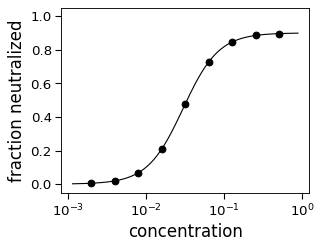
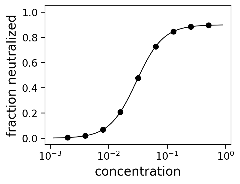
Now fit with infectivity_or_neutralized=’neutralized’, which is useful when the signal increases rather than decreases with increasing concentration (as would be the case if measuring fraction bound rather than fraction infectivity).

>>> neut_opp = HillCurve(cs, [1 - f for f in fs],
...                      fixtop=False, fixbottom=False,
...                      infectivity_or_neutralized='neutralized')
>>> numpy.allclose(neut_opp.top, 0.9, atol=1e-3)
True
>>> numpy.allclose(neut_opp.bottom, 0, atol=1e-3)
True
>>> numpy.allclose(neut_opp.midpoint, m)
True
>>> neut_opp.ic50() < neut_opp.midpoint
True
>>> fig, ax = neut_opp.plot(ylabel='fraction neutralized')

(png, hires.png, pdf)

For internal testing purposes, try with no_curve_fit_first=False.

>>> neut_ncf = HillCurve(cs, fs, fixbottom=False, no_curve_fit_first=True)
>>> numpy.allclose(neut_ncf.midpoint, m, atol=1e-4)
True
>>> numpy.allclose(neut_ncf.slope, s, atol=5e-3)
True
>>> numpy.allclose(neut_ncf.top, t, atol=1e-4)
True
>>> numpy.allclose(neut_ncf.bottom, b, atol=1e-3)
True

>>> neut_bounds_cover_ncf = HillCurve(
...     cs,
...     fs,
...     fixbottom=(0, 0.2),
...     fixtop=(0.9, 1),
...     fixslope=(1, 2),
...     no_curve_fit_first=True,
... )
>>> numpy.allclose(neut_bounds_cover_ncf.midpoint, m, atol=1e-4)
True
>>> numpy.allclose(neut_bounds_cover_ncf.slope, s, atol=1e-3)
True
>>> numpy.allclose(neut_bounds_cover_ncf.top, t, atol=1e-4)
True
>>> numpy.allclose(neut_bounds_cover_ncf.bottom, b, atol=1e-3)
True
>>> round(neut_bounds_cover_ncf.r2, 3)
1.0

>>> neut_bounds_nocover_ncf = HillCurve(
...     cs,
...     fs,
...     fixbottom=(0, 0.05),
...     fixtop=(0.9, 0.95),
...     fixslope=(1, 1.5),
...     no_curve_fit_first=True,
... )
>>> round(neut_bounds_nocover_ncf.midpoint, 2)
0.04
>>> round(neut_bounds_nocover_ncf.slope, 2)
1.5
>>> round(neut_bounds_nocover_ncf.top, 2)
0.95
>>> round(neut_bounds_nocover_ncf.bottom, 2)
0.05
>>> round(neut_bounds_nocover_ncf.r2, 2)
0.99

dataframe(concentrations='auto', extend=0.1)

Get data frame with curve data for plotting.

Useful if you want to get both the points and the fit curve to plot.

Args:

concentrations (array-like or ‘auto’ or ‘measured’)

Concentrations for which we compute the fit values. If ‘auto’ the automatically computed from data range using concentrationRange(). If ‘measured’ then only include measured values.

extend (float)

The value passed to concentrationRange() if concentrations is ‘auto’.

Returns:

A pandas DataFrame with the following columns:

• ‘concentration’: concentration

• ‘fit’: curve fit value at this point

• ‘measurement’: value of measurement at this point, or numpy.nan if no measurement here.

• ‘stderr’: standard error of measurement if provided.

static evaluate(c, m, s, b, t, infectivity_or_neutralized='infectivity')

\(f\left(c\right) = b + \frac{t-b}{1+\left(c/m\right)^s}\).

If infectivity_or_neutralized is ‘neutralized’ rather than ‘infectivity’, instead return \(f\left(c\right) = t + \frac{b-t}{1+\left(c/m\right)^s}\).

fracinfectivity(c)

Fraction infectivity at c for fitted parameters.

ic50(method='interpolate')

IC50 value.

Concentration where infectivity remaining is 0.5. Equals midpoint if and only if top = 1 and bottom = 0. Calculated from \(0.5 = b + \frac{t - b}{1 + (ic50/m)^s}\), which solves to \(ic50 = m \times \left(\frac{t - 0.5}{0.5 - b}\right)^{1/s}\)

Args:

method (str)

Can have following values:

• ‘interpolate’: only return a number for IC50 if it is in range of concentrations, otherwise return None.

• ‘bound’: if IC50 is out of range of concentrations, return upper or lower measured concentration depending on if IC50 is above or below range of concentrations. Assumes infectivity decreases with concentration.

Returns:

Number giving IC50 or None (depending on value of method).

ic50_bound()

Is IC50 ‘interpolated’, or an ‘upper’ or ‘lower’ bound.

ic50_stdev()

Get standard deviation of fit IC50 parameter.

Calculated just from estimated standard deviation on midpoint. Note if you have replicates, we recommend fitting separately and calculating standard error from those fits rather than using this value.

Returns:

A number giving the standard deviation, or None if cannot be estimated or if IC50 is at bound.

ic50_str(precision=3)

IC50 as string indicating upper / lower bounds with > or <.

Args:

Number of significant digits in returned string.

icXX(fracneut, *, method='interpolate')

Generalizes HillCurve.ic50() to arbitrary frac neutralized.

For instance, set fracneut to 0.95 if you want the IC95, the concentration where 95% is neutralized.

Args:

fracneut (float)

Compute concentration at which fracneut of the virus is expected to be neutralized. Note that this is the expected fraction neutralized, not the fraction infectivity.

method (str)

Can have following values:

• ‘interpolate’: only return a number for ICXX if it is in range of concentrations, otherwise return None.

• ‘bound’: if ICXX is out of range of concentrations, return upper or lower measured concentration depending on if ICXX is above or below range of concentrations. Assumes infectivity decreases with concentration.

Returns:

Number giving ICXX or None (depending on value of method).

icXX_bound(fracneut)

Like HillCurve.ic50_bound() for arbitrary frac neutralized.

icXX_str(fracneut, *, precision=3)

Like HillCurve.ic50_str() for arbitrary frac neutralized.

plot(*, concentrations='auto', ax=None, xlabel='concentration', ylabel='fraction infectivity', color='black', marker='o', markersize=6, linewidth=1, linestyle='-', yticklocs=None, draw_in_bounds=False)

Plot the neutralization curve.

Args:

concentrations

Concentrations to plot, same meaning as for HillCurve.dataframe().

ax (None or matplotlib axes.Axes object)

Use to plot on an existing axis. If using an existing axis, do not re-scale the axis limits to the data.

xlabel (str or None)

Label for x-axis.

ylabel (str or None)

Label for y-axis.

color (str)

Color of line and point.

marker (str)

Marker shape: https://matplotlib.org/api/markers_api.html

markersize (float)

Size of point marker.

linewidth (float)

Width of line.

linestyle (str)

Line style.

yticklocs (None or list)

Exact locations to place yticks; None means auto-locate.

draw_in_bounds (bool)

By default, the plotted curve extends a bit outside the actual data points on both sides. If this is set to True, then the plotted curve stops at the bounds of the data points.

Returns:

The 2-tuple (fig, ax) giving the matplotlib figure and axis.

exception neutcurve.hillcurve.HillCurveFittingError

Bases: Exception

Error fitting a HillCurve.

neutcurve.hillcurve.concentrationRange(bottom, top, npoints=200, extend=0.1)

Logarithmically spaced concentrations for plotting.

Useful if you want to plot a curve by fitting values to densely sampled points and need the concentrations at which to compute these points.

Args:

bottom (float)

Lowest concentration.

top (float)

Highest concentration.

npoints (int)

Number of points.

extend (float)

After transforming to log space, extend range of points by this much below and above bottom and top.

Returns:

A numpy array of npoints concentrations.

>>> numpy.allclose(concentrationRange(0.1, 100, 10, extend=0),
...                [0.1, 0.22, 0.46, 1, 2.15, 4.64, 10, 21.54, 46.42, 100],
...                atol=1e-2)
True
>>> numpy.allclose(concentrationRange(0.1, 100, 10),
...                [0.05, 0.13, 0.32, 0.79, 2.00, 5.01,
...                 12.59, 31.62, 79.43, 199.53],
...                atol=1e-2)
True