Lassa virus glycoprotein PacBio sequencing
This example shows how to use alignparse to process circular consensus sequences that map to multiple different targets. Here, our two targets are a wildtype and a codon optimized sequence for the Lassa virus (LASV) glycoprotein from the Josiah strain. For such targets we do not expect large internal deletions, so we use alignment settings optimized for codon-level mutations as these will be the settings used when analyzing mutant LASV GP sequences in later experiments.
Here we analyze a snippet of the full data set of circular consensus sequences so that the example is small and fast.
In the other included example notebooks (RecA deep mutational scanning libraries and Single-cell virus sequencing), we align and parse the PacBio reads using the single align_and_parse function. Here we use separate functions to do the aligning and parsing steps. This illustrates an additional use case and shows how this package could be used to parse alignments generated elsewhere as long as they have a cs tag and are in the SAM file format.
Set up for analysis
Import necessary Python modules:
[1]:
import os
import tempfile
import warnings

import Bio.SeqIO

import pandas as pd
import numpy

from plotnine import *

import pysam

import alignparse.ccs
import alignparse.minimap2
import alignparse.targets
import alignparse.cs_tag
import alignparse.consensus
Suppress warnings that clutter output:
[2]:
warnings.simplefilter("ignore")
Directory for output:
[3]:
outdir = "./output_files/"
os.makedirs(outdir, exist_ok=True)
Color palette for plots:
[4]:
CBPALETTE = ("#999999", "#E69F00", "#56B4E9", "#009E73")
Target amplicons
We have performed sequencing of several LASV GP amplicons that include the glycoprotein sequence along with a PacBio index and several other features. Here we analyze reads mapping to two of these amplicons. The amplicons are defined in Genbank Flat File format. If there are multiple targets, they can all be defined in a single Genbank file (as we did in the Single-cell virus sequencing example) or each target can be defined in its own Genbank file (as we’ve done here).
First, let’s just look at the files:
[5]:
target_file_names = ["LASV_Josiah_WT", "LASV_Josiah_OPT"]

targetfiles = [
    f"input_files/{target_file_name}.gb" for target_file_name in target_file_names
]

for targetfile in targetfiles:
    with open(targetfile) as f:
        print(f.read())
LOCUS       LASV_Josiah_WT          1730 bp ds-DNA     linear       14-JUN-2019
DEFINITION  .
ACCESSION
VERSION
SOURCE      Kate Crawford
  ORGANISM  .
COMMENT     PacBio amplicon for LASV Josiah WT sequence
FEATURES             Location/Qualifiers
     T2A             85..147
                     /label="T2A"
     WPRE            1639..1730
                     /label="WPRE"
     ZsGreen         15..84
                     /label="ZsGreen"
     termini3        1639..1730
                     /label="3'Termini"
     index           9..14
                     /label="index"
     leader5         1..8
                     /label="5' leader"
     termini5        1..147
                     /label="5'Termini"
     variant_tag5    34..34
                     /variant_1=T
                     /variant_2=C
                     /label="5'VariantTag"
     variant_tag3    1702..1702
                     /variant_1=G
                     /variant_2=A
                     /label="3'VariantTag"
     spacer          1624..1638
                     /label="3'Spacer"
     gene            148..1623
                     /label="LASV_Josiah_WT"

ORIGIN
        1 GACTGATANN NNNNcagcga cgccaagaac cagYagtggc acctgaccga gcacgccatc
       61 gcctccggcT CCGCCTTGCC CGCTGGATCC GGCGAGGGCA GAGGAAGTCT GCTAACATGC
      121 GGTGACGTCG AGGAGAATCC TGGCCCAATG GGACAAATAG TGACATTCTT CCAGGAAGTG
      181 CCTCATGTAA TAGAAGAGGT GATGAACATT GTTCTCATTG CACTGTCTGT ACTAGCAGTG
      241 CTGAAAGGTC TGTACAATTT TGCAACGTGT GGCCTTGTTG GTTTGGTCAC TTTCCTCCTG
      301 TTGTGTGGTA GGTCTTGCAC AACCAGTCTT TATAAAGGGG TTTATGAGCT TCAGACTCTG
      361 GAACTAAACA TGGAGACACT CAATATGACC ATGCCTCTCT CCTGCACAAA GAACAACAGT
      421 CATCATTATA TAATGGTGGG CAATGAGACA GGACTAGAAC TGACCTTGAC CAACACGAGC
      481 ATTATTAATC ACAAATTTTG CAATCTGTCT GATGCCCACA AAAAGAACCT CTATGACCAC
      541 GCTCTTATGA GCATAATCTC AACTTtccac ttgtccatcc ccaacTTCAA TCAGTATGAG
      601 GCAATGAGCT GCGATTTTAA TGGGGGAAAG ATTAGTGTGC AGTACAACCT GAGTCACAGC
      661 TATGCTGGGG ATGCAGCCAA CCATTGTGGT ACTGTTGCAA ATGGTGTGTT ACAGACTTTT
      721 ATGAGGATGG CTTGGGGTGG GAGCTACATT GCTCTTGACT CAGGCCGTGG CAACTGGGAC
      781 TGTATTATGA CTAGTTATCA ATATCTGATA ATCCAAAATA CAACCTGGGA AGATCACTGC
      841 CAATTCTCGA GACCATCTCC CATCGGTTAT CTCGGGCTCC TCTCACAAAG GACTAGAGAT
      901 ATTTATATTA GTAGAAGATT GCTAGGCACA TTCACATGGA CACTGTCAGA TTCTGAAGGT
      961 AAAGACACAC CAGGGGGATA TTGTCTGACC AGGTGGATGC TAATTGAGGC TGAACTAAAA
     1021 TGCTTCGGGA ACACAGCTGT GGCAAAATGT AATGAGAAGC ATGATGAgga attttgtgac
     1081 atgctgaggc TGTTTGACTT CAACAAACAA GCCATTCAAA GGTTGAAAGC TGAAGCACAA
     1141 ATGAGCATTC AGTTGATCAA CAAAGCAGTA AATGCTTTGA TAAATGACCA ACTTATAATG
     1201 AAGAACCATC TACGGGACAT CATGGGAATT CCATACTGTA ATTACAGCAA GTATTGGTAC
     1261 CTCAACCACA CAACTACTGG GAGAACATCA CTGCCCAAAT GTTGGCTTGT ATCAAATGGT
     1321 TCATACTTGA ACGAGACCCA CTTTTCTGAT GATATTGAAC AACAAGCTGA CAATATGATC
     1381 ACTGAGATGT TACAGAAGGA GTATATGGAG AGGCAGGGGA AGACACCATT GGGTCTAGTT
     1441 GACCTCTTTG TGTTCAGCAC AAGTTTCTAT CTTATTAGCA TCTTCCTTCA CCTAGTCAAA
     1501 ATACCAACTC ATAGGCATAT TGTAGGCAAG TCGTGTCCCA AACCTCACAG ATTGAATCAT
     1561 ATGGGCATTT GTTCCTGTGG ACTCTACAAA CAGCCTGGTG TGCCTGTGAA ATGGAAGAGA
     1621 TGAGCTAGCT AAACGCGTTG ATCCtaatca acctctggat tacaaaattt gtgaaagatt
     1681 gactggtatt cttaactatg tRgctccttt tacgctatgt ggatacgctg
//

LOCUS       LASV_Josiah_OPT          1730 bp ds-DNA     linear       14-JUN-2019
DEFINITION  .
ACCESSION
VERSION
SOURCE      Kate Crawford
  ORGANISM  .
COMMENT     PacBio amplicon for LASV Josiah OPT sequence
FEATURES             Location/Qualifiers
     T2A             85..147
                     /label="T2A"
     WPRE            1639..1730
                     /label="WPRE"
     ZsGreen         15..84
                     /label="ZsGreen"
     termini3        1639..1730
                     /label="3'Termini"
     index           9..14
                     /label="index"
     leader5         1..8
                     /label="5' leader"
     termini5        1..147
                     /label="5'Termini"
     variant_tag5     34..34
                     /variant_1=T
                     /variant_2=C
                     /label="5'VariantTag"
     variant_tag3     1702..1702
                     /variant_1=G
                     /variant_2=A
                     /label="3'VariantTag"
     spacer          1624..1638
                     /label="3'Spacer"
     gene            148..1623
                     /label="LASV_Josiah_OPT"

ORIGIN
        1 GACTGATANN NNNNcagcga cgccaagaac cagYagtggc acctgaccga gcacgccatc
       61 gcctccggcT CCGCCTTGCC CGCTGGATCC GGCGAGGGCA GAGGAAGTCT GCTAACATGC
      121 GGTGACGTCG AGGAGAATCC TGGCCCAATG GGCCAGATCG TGACCTTCTT CCAAGAAGTG
      181 CCTCATGTGA TTGAGGAGGT GATGAATATC GTGCTGATCG CTTTAAGCGT GCTGGCCGTT
      241 CTTAAGGGCC TCTATAACTT CGCCACTTGT GGTTTAGTCG GACTGGTGAC ATTTCTGCTG
      301 CTGTGTGGCA GATCTTGTAC CACATCTTTA TACAAGGGCG TGTACGAGCT GCAGACTTTA
      361 GAACTGAACA TGGAGACTTT AAACATGACC ATGCCTTTAA GCTGTACCAA GAACAATAGC
      421 CACCACTACA TCATGGTGGG CAACGAGACC GGTTTAGAAC TGACACTCAC CAACACCAGC
      481 ATTATCAACC ATAAGTTCTG CAACCTCTCC GACGCTCACA AGAAGAATTT ATACGACCAC
      541 GCTTTAATGA GCATCATCTC CACCTTCCAT CTCTCCATTC CTAATttcaa ccagtacgag
      601 gccatgAGCT GCGACTTTAA CGGCGGCAAG ATCTCCGTGC AGTACAATTT ATCCCATAGC
      661 TACGCCGGCG ATGCCGCCAA TCACTGCGGA ACCGTGGCCA ACGGCGTGCT GCAGACATTC
      721 ATGAGGATGG CTTGGGGCGG CTCCTATATC GCTTTAGACT CCGGCAGAGG AAACTGGGAC
      781 TGTATCATGA CCAGCTACCA ATATTTAATC ATTCAGAACA CCACATGGGA GGACCACTGC
      841 CAATTCTCTC GTCCCTCTCC TATCGGCTAT CTGGGACTGC TGTCCCAGAG GACCAGAGAC
      901 ATCTACATCT CTCGTAGGCT GCTGGGCACA TTCACTTGGA CTTTAAGCGA CAGCGAAGGC
      961 AAAGATACTC CCGGTGGCTA CTGTTTAACA AGATGGATGC TGATCGAGGC CGAGCTCAAG
     1021 TGCTTCGGAA ATACCGCCGT GGCCAAATGC AACGAGAAAC ACGACGAGGA GTTCTGCGAC
     1081 ATGCTGAGGC TCTTCGACTT CAacaagcaa gccattcaga ggcTGAAGGC CGAAGCCCAG
     1141 ATGTCCATCC AGCTGATTAA TAAGGCCGTG AATGCCCTCA TTAACGACCA GCTGATCATG
     1201 AAGAACCATT TAAGGGACAT CATGGGCATC CCTTATTGCA ACTACAGCAA ATACTGGTAT
     1261 TTAAATCATA CCACCACCGG TCGTACATCC TTACCTAAGT GCTGGCTGGT CAGCAATGGC
     1321 TCCTATTTAA ACGAGACACA CTTCTCCGAC GACATCGAGC AGCAAGCCGA CAACATGATC
     1381 ACCGAAATGC TCCAGAAGGA GTACATGGAG AGGCAAGGTA AGACTCCTCT GGGTTTAGTG
     1441 GATTTATTCG TCTTCAGCAC CTCCTTCTAT TTAATCTCCA TCTTTCTTCA TCTGGTGAAG
     1501 ATTCCTACCC ACAGACACAT TGTGGGCAAG AGCTGTCCTA AGCCTCATAG ACTGAACCAC
     1561 ATGGGCATCT GTAGCTGCGG TTTATATAAA CAGCCCGGTG TTCCCGTTAA GTGGAAGAGG
     1621 TGAGCTAGCT AAACGCGTTG ATCCtaatca acctctggat tacaaaattt gtgaaagatt
     1681 gactggtatt cttaactatg tRgctccttt tacgctatgt ggatacgctg
//
Along with the Genbank files giving the sequences of the amplicons, we have a YAML file specifying how to filter and parse alignments to these amplicons.
Below is the text of the YAML file.
Additional information about these filters can be found in the RecA deep mutational scanning libraries example notebook or the Targets documentation.
A filter setting of null indicates this filter is not applied. When filters are missing for a feature, they are automatically set to zero.
Here we filter the gene based on mutation_op_counts by setting the mutation_nt_counts filter for the gene to null. Although we do not expect these sequences to have large indels, we want to confirm this. Filtering on mutation “operations” allows us to retain sequences with large indels by only filtering on the number of indels, not the number of nucleotides inserted or deleted. Overall, this example uses very loose filters to allow us to do further analyses of the types of
mutations that are arising in these samples.
The YAML file also specifies what information is parsed from alignments that are not filtered out. As you can see, for some features we parse the mutations or the full sequence of the feature, along with the accuracy of that feature in the sequencing query (computed from the Q-values).
As seen below, we can use YAML syntax to apply one set of filters to multiple targets. Here, we apply the same filters to both targets, but this is not necessary.
[6]:
lasv_parse_specs_file = "input_files/lasv_feature_parse_specs.yaml"
with open(lasv_parse_specs_file) as f:
    print(f.read())
LASV_Josiah_WT: &LASV_target_parse_specs
  query_clip5: 10
  query_clip3: 10
  termini5:
    filter:
      clip5: 10
      mutation_nt_count: 5
      mutation_op_count: null
  termini3:
    filter:
      clip3: 10
      mutation_nt_count: 5
      mutation_op_count: null
  gene:
    filter:
      mutation_nt_count: null
      mutation_op_count: 30
    return: [mutations, accuracy]
  spacer:
    filter:
      mutation_nt_count: 1
      mutation_op_count: null
  index:
    return: sequence
  variant_tag5:
    return: sequence
  variant_tag3:
    return: sequence

LASV_Josiah_OPT: *LASV_target_parse_specs
Read the amplicons in feature_parse_specs into a Targets object, specifying the features that we require the target to contain. The Targets in this example have more features specified in their Genbank files than we want to parse, so we set allow_extra_features to True.
[7]:
targets = alignparse.targets.Targets(
    seqsfile=targetfiles,
    feature_parse_specs=lasv_parse_specs_file,
    allow_extra_features=True,
)
When we look at the targets.feature_parse_specs, we now see that the previously unspecified specs have been filled in with the defaults.
[8]:
print(targets.feature_parse_specs("yaml"))
LASV_Josiah_WT: &id001
  query_clip5: 10
  query_clip3: 10
  termini5:
    filter:
      clip5: 10
      mutation_nt_count: 5
      mutation_op_count: null
      clip3: 0
    return: []
  termini3:
    filter:
      clip3: 10
      mutation_nt_count: 5
      mutation_op_count: null
      clip5: 0
    return: []
  gene:
    filter:
      mutation_nt_count: null
      mutation_op_count: 30
      clip5: 0
      clip3: 0
    return:
    - mutations
    - accuracy
  spacer:
    filter:
      mutation_nt_count: 1
      mutation_op_count: null
      clip5: 0
      clip3: 0
    return: []
  index:
    return:
    - sequence
    filter:
      clip5: 0
      clip3: 0
      mutation_nt_count: 0
      mutation_op_count: 0
  variant_tag5:
    return:
    - sequence
    filter:
      clip5: 0
      clip3: 0
      mutation_nt_count: 0
      mutation_op_count: 0
  variant_tag3:
    return:
    - sequence
    filter:
      clip5: 0
      clip3: 0
      mutation_nt_count: 0
      mutation_op_count: 0
LASV_Josiah_OPT: *id001
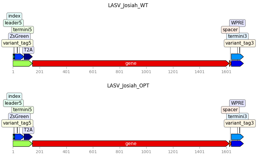
We can also plot the Targets. All features specified in the targets’ Genbank files will be annotated, even if they are not in feature_parse_specs.
[9]:
_ = targets.plot(ax_width=10)
Note that if needed, it is also possible to get a Targets object for just some of the sequences specified in seqsfile or feature_parse_specs. This is most commonly useful when seqsfile contains additional sequences that are not of interest. Below we illustrate how to do this by:
Setting
select_target_namesto only keep the LASV_Josiah_WT sequence inseqsfileSetting
ingore_feature_parse_specsto ignore the other targets (in this case, LASV_Josiah_OPT) infeature_parse_specs
[10]:
targets_subset = alignparse.targets.Targets(
    seqsfile=targetfiles,
    feature_parse_specs=lasv_parse_specs_file,
    allow_extra_features=True,
    select_target_names=["LASV_Josiah_WT"],
    ignore_feature_parse_specs_keys=["LASV_Josiah_OPT"],
)

print(f"Here are the names of the retained targets: {targets_subset.target_names}")
Here are the names of the retained targets: ['LASV_Josiah_WT']
PacBio CCSs
We will align PacBio circular consensus sequences (CCSs) to the target. First, we want to look at the CCSs. A FASTQ file with these CCSs along with an associated report file were generated using the PacBio ccs program (see here for details on ccs) using commands like the following (generates report file and BAM of CCSs):
ccs --minLength 50 --maxLength 5000 \
    --minPasses 3  --minPredictedAccuracy 0.999 \
    --reportFile lasv_pilot_report.txt \
    --polish --numThreads 16 \
    lasv_pilot_subreads.bam lasv_pilot_ccs.bam
The BAM file was then converted to a FASTQ file using samtools with flags to retain the number of passes (np) and read quality (rq). Here we convert the BAM file to a gzipped FASTQ file to demonstrate the use of compressed files:
samtools bam2fq -T np,rq lasv_pilot_ccs.bam | gzip > lasv_pilot_ccs.fastq.gz
Here is a data frame with the resulting FASTQ and BAM files:
[11]:
run_names = ["lasv_pilot"]
ccs_dir = "input_files"
file_name = "lasv_example"

pacbio_runs = pd.DataFrame(
    {
        "name": run_names,
        "report": [f"{ccs_dir}/{name}_report.txt" for name in run_names],
        "fastq": [f"{ccs_dir}/{file_name}_ccs.fastq.gz"],
    }
)

pacbio_runs
[11]:
| name | report | fastq | |
|---|---|---|---|
| 0 | lasv_pilot | input_files/lasv_pilot_report.txt | input_files/lasv_example_ccs.fastq.gz |
We create a Summaries object for these CCSs:
[12]:
ccs_summaries = alignparse.ccs.Summaries(pacbio_runs)
Plot how many ZMWs yielded CCSs:
[13]:
# NBVAL_IGNORE_OUTPUT

p = ccs_summaries.plot_zmw_stats()
_ = p.draw()
[14]:
ccs_summaries.zmw_stats()
[14]:
| name | status | number | fraction | |
|---|---|---|---|---|
| 0 | lasv_pilot | Success -- CCS generated | 250 | 0.4996 |
| 1 | lasv_pilot | Failed -- Not enough full passes | 157 | 0.3144 |
| 2 | lasv_pilot | Failed -- CCS below minimum predicted accuracy | 86 | 0.1720 |
| 3 | lasv_pilot | Failed -- No usable subreads | 6 | 0.0137 |
| 4 | lasv_pilot | Failed -- Other reason | 0 | 0.0000 |
Statistics on the CCSs (length, number of subread passes, accuracy):
[15]:
# NBVAL_IGNORE_OUTPUT

for stat in ["length", "passes", "accuracy"]:
    if ccs_summaries.has_stat(stat):
        p = ccs_summaries.plot_ccs_stats(stat)
        _ = p.draw()
    else:
        print(f"No information available on CCS {stat}")
Align CCSs to target
Now we use minimap2 to align the CCSs to the target.
First, we create a Mapper object to run minimap2, using the options for codon-level deep mutational scanning (specified by alignparse.minimap2.OPTIONS_CODON_DMS):
[16]:
# NBVAL_IGNORE_OUTPUT

mapper = alignparse.minimap2.Mapper(alignparse.minimap2.OPTIONS_CODON_DMS)

print(
    f"Using `minimap2` {mapper.version} with these options:\n"
    + " ".join(mapper.options)
)
Using `minimap2` 2.22-r1101 with these options:
-A2 -B4 -O12 -E2 --end-bonus=13 --secondary=no --cs
Now use this mapper to do the alignments to a SAM file. First, add the names of the desired alignment files to our data frame:
[17]:
pacbio_runs = pacbio_runs.assign(
    alignments=lambda x: outdir + x["name"] + "_alignments.sam"
)

pacbio_runs
[17]:
| name | report | fastq | alignments | |
|---|---|---|---|---|
| 0 | lasv_pilot | input_files/lasv_pilot_report.txt | input_files/lasv_example_ccs.fastq.gz | ./output_files/lasv_pilot_alignments.sam |
Now we run targets.align using the mapper to actually align the FASTQ queries to the target:
[18]:
for tup in pacbio_runs.itertuples(index=False):
    print(f"Aligning {tup.fastq} to create {tup.alignments}...")
    targets.align(queryfile=tup.fastq, alignmentfile=tup.alignments, mapper=mapper)
Aligning input_files/lasv_example_ccs.fastq.gz to create ./output_files/lasv_pilot_alignments.sam...
These SAM files now contain the alignments along with the cs tag.
An example cs tag is:
[19]:
for fname in pacbio_runs["alignments"][:1]:
    with pysam.AlignmentFile(fname) as f:
        a = next(f)
        print(f"First alignment in {fname} has `cs` tag:\n" + a.get_tag("cs"))
First alignment in ./output_files/lasv_pilot_alignments.sam has `cs` tag:
:8*ng*na*ng*na*nc*ng:19*nc:1667*na:28
Parse the alignments
Now we use Targets.parse_alignments to parse the SAM files to get the information we specified for return. This function returns a data frame (readstats) on the overall parsing stats, plus dicts keyed by the names of each target in Targets giving data frames of the aligned and filtered
reads. Here we return the aligned and filtered reads as dictionaries of data frames.
The aligned and filtered read information can instead be returned as CSV files containing these data frames by setting the to_csv argument to True. Note: When using the combined Targets.align_and_parse function as in the other example notebooks (RecA DMS libraries and Single-cell virus
sequencing), these CSV files will always be created, even if to_csv is False and the align_and_parse function is returning aligned and filtered as dictionaries of data frames in its final output.
Here we only have one PacBio run, but in practice we will often have multiple. As such, our example shows how to concatenate the readstats, aligned, and filtered data frames for each PacBio run and then look at the data frames together:
[20]:
readstats = []
aligned = {targetname: [] for targetname in targets.target_names}
filtered = {targetname: [] for targetname in targets.target_names}

for run in pacbio_runs.itertuples():
    print(f"Parsing PacBio run {run.name}")
    run_readstats, run_aligned, run_filtered = targets.parse_alignment(
        run.alignments, filtered_cs=True
    )

    # when concatenating add the run name to keep track of runs for results
    readstats.append(run_readstats.assign(run_name=run.name))
    for targetname in targets.target_names:
        aligned[targetname].append(run_aligned[targetname].assign(run_name=run.name))
        filtered[targetname].append(run_filtered[targetname].assign(run_name=run.name))

# now concatenate the data frames for each run
readstats = pd.concat(readstats, ignore_index=True, sort=False)
for targetname in targets.target_names:
    aligned[targetname] = pd.concat(aligned[targetname], ignore_index=True, sort=False)
    filtered[targetname] = pd.concat(
        filtered[targetname], ignore_index=True, sort=False
    )
Parsing PacBio run lasv_pilot
First lets look at the read stats:
From the known composition of the library, there should be more LASV_Josiah_OPT reads than LASV_Josiah_WT.
[21]:
readstats
[21]:
| category | count | run_name | |
|---|---|---|---|
| 0 | filtered LASV_Josiah_WT | 23 | lasv_pilot |
| 1 | aligned LASV_Josiah_WT | 84 | lasv_pilot |
| 2 | filtered LASV_Josiah_OPT | 32 | lasv_pilot |
| 3 | aligned LASV_Josiah_OPT | 111 | lasv_pilot |
| 4 | unmapped | 0 | lasv_pilot |
[22]:
# NBVAL_IGNORE_OUTPUT

p = (
    ggplot(readstats, aes("category", "count"))
    + geom_bar(stat="identity")
    + facet_wrap("~ run_name", nrow=1)
    + theme(
        axis_text_x=element_text(angle=90), figure_size=(1.5 * len(pacbio_runs), 2.5)
    )
)
_ = p.draw()
Now look at the information on the filtered reads. This is a bigger data frame, so we just look at the first few lines for the first target (of which there is only one anyway):
[23]:
filtered[targets.target_names[0]].head()
[23]:
| query_name | filter_reason | filter_cs | run_name | |
|---|---|---|---|---|
| 0 | m54228_190605_190010/4194989/ccs | termini5 clip5 | *nc*na*nc:19*nc:113 | lasv_pilot |
| 1 | m54228_190605_190010/4260241/ccs | index clip5 | *ng*na*nc*na*nc | lasv_pilot |
| 2 | m54228_190605_190010/4260334/ccs | query_clip5 | None | lasv_pilot |
| 3 | m54228_190605_190010/4391712/ccs | termini5 clip5 | lasv_pilot | |
| 4 | m54228_190605_190010/4456843/ccs | termini3 clip3 | lasv_pilot |
[24]:
# NBVAL_IGNORE_OUTPUT

for targetname in targets.target_names:
    target_filtered = filtered[targetname]
    nreasons = target_filtered["filter_reason"].nunique()
    p = (
        ggplot(target_filtered, aes("filter_reason"))
        + geom_bar()
        + facet_wrap("~ run_name", nrow=1)
        + labs(title=targetname)
        + theme(
            axis_text_x=element_text(angle=90),
            figure_size=(0.3 * nreasons * len(pacbio_runs), 2.5),
        )
    )
    _ = p.draw()
Error filtering
Before looking at the information for the validly aligned (not filtered) reads, it is important to get a sense of the error rate for these sequencing reads.
These reads do not have random barcodes on the initial viral entry protein plasmids, but we can use the gene_accuracy information output from constructing the ccss to examine accuracy.
We will do this using a similar method to that implemented in the RecA DMS libraries example notebook. However, here we will plot the graphs for each target.
We anticipate excluding all CCSs for which the error rate for either the gene or barcode is \(>10^{-4}\). We specify this cutoff below.
[25]:
# NBVAL_IGNORE_OUTPUT

error_rate_floor = 1e-7  # error rates < this set to this
error_cutoff = 1e-4

for targetname in targets.target_names:
    aligned[targetname] = aligned[targetname].assign(
        gene_error=lambda x: numpy.clip(1 - x["gene_accuracy"], error_rate_floor, None)
    )
    p = (
        ggplot(
            aligned[targetname].melt(
                id_vars=["run_name"],
                value_vars=["gene_error"],
                var_name="feature_type",
                value_name="error rate",
            ),
            aes("error rate"),
        )
        + geom_histogram(bins=25)
        + geom_vline(xintercept=error_cutoff, linetype="dashed", color=CBPALETTE[1])
        + facet_grid("~ feature_type")
        + theme(figure_size=(3, 3))
        + labs(y=("number of CCSs"), title=(targetname))
        + scale_x_log10()
    )

    _ = p.draw()
Next, we store all reads with an error rate \(<10^{-4}\) in new data frames for retained sequences.
We will use these retained sequences for further analyses.
[26]:
retained = {targetname: [] for targetname in targets.target_names}
for targetname in targets.target_names:
    target_retained = aligned[targetname][
        aligned[targetname]["gene_error"] <= error_cutoff
    ].reset_index(drop=True)
    retained[targetname] = target_retained
Data analysis
Now we can examine our data in more detail.
We will only display a few columns so the example renders well in the documentation. First, let’s look at the query_name, gene_mutations, and index_sequence columns for the first few entries in the retained data frame for each target:
[27]:
display_columns = ["query_name", "gene_mutations", "index_sequence"]
for target_name in targets.target_names:
    print(target_name)
    display(retained[target_name][display_columns].head())
LASV_Josiah_WT
| query_name | gene_mutations | index_sequence | |
|---|---|---|---|
| 0 | m54228_190605_190010/4194436/ccs | GGTATG | |
| 1 | m54228_190605_190010/4194472/ccs | T572C | GGTATG |
| 2 | m54228_190605_190010/4194509/ccs | GGTATG | |
| 3 | m54228_190605_190010/4194553/ccs | GGTATG | |
| 4 | m54228_190605_190010/4194576/ccs | AGACAC |
LASV_Josiah_OPT
| query_name | gene_mutations | index_sequence | |
|---|---|---|---|
| 0 | m54228_190605_190010/4194382/ccs | GAGACG | |
| 1 | m54228_190605_190010/4194390/ccs | ACGACC | |
| 2 | m54228_190605_190010/4194399/ccs | ACGACC | |
| 3 | m54228_190605_190010/4194439/ccs | ACGACC | |
| 4 | m54228_190605_190010/4194445/ccs | CTTCAC |
As seen by the index_sequence columns, each target here has 2 or 3 different indices that map to it. These indicies indicate different samples.
We can then split these data frames into sample-specific data frames based on the known starting index sequences for each target. We will store these data frames in a new dictionary, keyed by target and index.
[28]:
indices = {
    "LASV_Josiah_WT": ["AGACAC", "GGTATG"],
    "LASV_Josiah_OPT": ["ACGACC", "CTTCAC", "GAGACG"],
}
target_idx_retained = {}
index_counts = {target: [] for target in indices}
index_counts_dfs = {}
for target_name in targets.target_names:
    for index in indices[target_name]:
        target_idx_retained[f"{target_name}_{index}"] = retained[target_name][
            retained[target_name]["index_sequence"] == index
        ].reset_index(drop=True)
        index_counts[f"{target_name}"].append(
            (index, len(target_idx_retained[f"{target_name}_{index}"]))
        )
    index_counts[f"{target_name}"].append(
        (
            "invalid",
            (
                len(retained[target_name])
                - sum(idx_tup[1] for idx_tup in index_counts[target_name])
            ),
        )
    )
    index_counts_dfs[target_name] = pd.DataFrame(
        index_counts[target_name], columns=["index", "count"]
    )
In the process of making these separate data frames, we also kept track of how many reads for each target map to each index or don’t map to an index (so have an ‘invalid’ index) and can now plot these counts. As seen below, only one sequence in this example has an invalid index and it maps to the LASV_Josiah_OPT target.
[29]:
# NBVAL_IGNORE_OUTPUT

for target_name in targets.target_names:
    df = index_counts_dfs[target_name]
    df["target"] = [target_name] * len(df)
    id_order = ["invalid"] + df["index"][:-1].to_list()
    df["index"] = pd.Categorical(df["index"], categories=id_order, ordered=True)
    index_count_plot = (
        ggplot(df, aes(x="target", y="count", fill="index"))
        + geom_bar(stat="identity", position="stack")
        + scale_fill_manual(values=CBPALETTE)
        + theme(
            axis_text_x=element_text(angle=90, vjust=1, hjust=0.5), figure_size=(1, 2)
        )
        + ylab("Reads")
        + xlab("Target")
        + ggtitle("Reads per Sample Index")
    )

    _ = index_count_plot.draw()
The two target-specific data frames are now five index-specific data frames. Again we will display the query_name, gene_mutations, and index_sequence columns.
[30]:
for target_idx in target_idx_retained:
    print(target_idx)
    display(target_idx_retained[target_idx][display_columns].head(3))
LASV_Josiah_WT_AGACAC
| query_name | gene_mutations | index_sequence | |
|---|---|---|---|
| 0 | m54228_190605_190010/4194576/ccs | AGACAC | |
| 1 | m54228_190605_190010/4194612/ccs | AGACAC | |
| 2 | m54228_190605_190010/4194613/ccs | AGACAC |
LASV_Josiah_WT_GGTATG
| query_name | gene_mutations | index_sequence | |
|---|---|---|---|
| 0 | m54228_190605_190010/4194436/ccs | GGTATG | |
| 1 | m54228_190605_190010/4194472/ccs | T572C | GGTATG |
| 2 | m54228_190605_190010/4194509/ccs | GGTATG |
LASV_Josiah_OPT_ACGACC
| query_name | gene_mutations | index_sequence | |
|---|---|---|---|
| 0 | m54228_190605_190010/4194390/ccs | ACGACC | |
| 1 | m54228_190605_190010/4194399/ccs | ACGACC | |
| 2 | m54228_190605_190010/4194439/ccs | ACGACC |
LASV_Josiah_OPT_CTTCAC
| query_name | gene_mutations | index_sequence | |
|---|---|---|---|
| 0 | m54228_190605_190010/4194445/ccs | CTTCAC | |
| 1 | m54228_190605_190010/4194501/ccs | CTTCAC | |
| 2 | m54228_190605_190010/4194549/ccs | CTTCAC |
LASV_Josiah_OPT_GAGACG
| query_name | gene_mutations | index_sequence | |
|---|---|---|---|
| 0 | m54228_190605_190010/4194382/ccs | GAGACG | |
| 1 | m54228_190605_190010/4194467/ccs | GAGACG | |
| 2 | m54228_190605_190010/4194491/ccs | GAGACG |
We can add mutation info for the genes in these targets using alignparse.consensus.add_mut_info_cols.
[31]:
for target_idx in target_idx_retained:
    target_idx_retained[target_idx] = alignparse.consensus.add_mut_info_cols(
        target_idx_retained[target_idx],
        mutation_col="gene_mutations",
        n_sub_col="n_gene_subs",
        n_indel_col="n_gene_indels",
    )
We can then plot the number of reads for each sample that has each number of substitutions or indels to get a sense of how many mutations are in these reads, if some smaples have more mutations than others, and if substitutions or indels are more prevalent in these sequences.
With such a small sample snippet of the data, it is difficult to make any conclusions, but with a full dataset, this can provide important information about the mutational processes at work for each sample.
[32]:
# NBVAL_IGNORE_OUTPUT

mut_cols = ["n_gene_subs", "n_gene_indels"]
for target_idx in target_idx_retained:
    target_idx_plot_muts = target_idx_retained[target_idx][mut_cols].melt()
    mut_counts_plot = (
        ggplot(target_idx_plot_muts, aes("value"))
        + geom_bar()
        + facet_wrap("~ variable", ncol=2)
        + xlim(-0.5, 2.5)
        + labs(title=f"{target_idx}")
        + theme(
            axis_text_x=element_text(angle=90),
            figure_size=(3, 2.5),
        )
    )
    _ = mut_counts_plot.draw()