RecA deep mutational scanning libraries

This example shows how to use alignparse to process PacBio circular consensus sequencing of a barcoded library of RecA variants for deep mutational scanning.

Set up for analysis

Import necessary Python modules. We use alignparse for most of the operations, plotnine for ggplot2-like plotting, and a few functitons from dms_variants:

import os
import warnings

import numpy

import pandas as pd

from plotnine import *

import alignparse.ccs
import alignparse.consensus
import alignparse.minimap2
import alignparse.targets
from alignparse.constants import CBPALETTE

import dms_variants.utils

Suppress warnings that clutter output:

warnings.simplefilter("ignore")

Directory for output:

outdir = "./output_files/"
os.makedirs(outdir, exist_ok=True)

Target amplicon

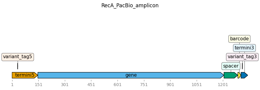
We have performed sequencing of an amplicon that includes the RecA gene along with barcodes and several other features. The amplicon is defined in Genbank Flat File format. First, let’s look at that file. Note how it defines the features; this is how they must be defined to be handled by alignparse. Note also how there are ambiguous nucleotides in the barcode and variant tag regions:

recA_targetfile = "input_files/recA_amplicon.gb"

with open(recA_targetfile) as f:
    print(f.read())

LOCUS       RecA_PacBio_amplicon    1342 bp ds-DNA     linear       06-AUG-2018
DEFINITION  PacBio amplicon for deep mutational scanning of E. coli RecA.
ACCESSION   None
VERSION
SOURCE      Danny Lawrence
  ORGANISM  .
COMMENT     PacBio amplicon for RecA libraries.
COMMENT     There are single nucleotide tags in the 5' and 3' termini to measure strand exchange.
FEATURES             Location/Qualifiers
     termini5        1..147
                     /label="termini 5' of gene"
     gene            148..1206
                     /label="RecA gene"
     spacer          1207..1285
                     /label="spacer between gene & barcode"
     barcode         1286..1303
                     /label="18 nucleotide barcode"
     termini3        1304..1342
                     /label="termini 3' of barcode"
     variant_tag5    33..33
                     /label="5' variant tag"
     variant_tag3    1311..1311
                     /label="3' variant tag"
ORIGIN
        1 gcacggcgtc acactttgct atgccatagc atRtttatcc ataagattag cggatcctac
       61 ctgacgcttt ttatcgcaac tctctactgt ttctccataa cagaacatat tgactatccg
      121 gtattacccg gcatgacagg agtaaaaATG GCTATCGACG AAAACAAACA GAAAGCGTTG
      181 GCGGCAGCAC TGGGCCAGAT TGAGAAACAA TTTGGTAAAG GCTCCATCAT GCGCCTGGGT
      241 GAAGACCGTT CCATGGATGT GGAAACCATC TCTACCGGTT CGCTTTCACT GGATATCGCG
      301 CTTGGGGCAG GTGGTCTGCC GATGGGCCGT ATCGTCGAAA TCTACGGACC GGAATCTTCC
      361 GGTAAAACCA CGCTGACGCT GCAGGTGATC GCCGCAGCGC AGCGTGAAGG TAAAACCTGT
      421 GCGTTTATCG ATGCTGAACA CGCGCTGGAC CCAATCTACG CACGTAAACT GGGCGTCGAT
      481 ATCGACAACC TGCTGTGCTC CCAGCCGGAC ACCGGCGAGC AGGCACTGGA AATCTGTGAC
      541 GCCCTGGCGC GTTCTGGCGC AGTAGACGTT ATCGTCGTTG ACTCCGTGGC GGCACTGACG
      601 CCGAAAGCGG AAATCGAAGG CGAAATCGGC GACTCTCATA TGGGCCTTGC GGCACGTATG
      661 ATGAGCCAGG CGATGCGTAA GCTGGCGGGT AACCTGAAGC AGTCCAACAC GCTGCTGATC
      721 TTCATCAACC AGATCCGTAT GAAAATTGGT GTGATGTTCG GCAACCCGGA AACCACTACC
      781 GGTGGTAACG CGCTGAAATT CTACGCCTCT GTTCGTCTCG ACATCCGTCG TATCGGCGCG
      841 GTGAAAGAGG GCGAAAACGT GGTGGGTAGC GAAACCCGCG TGAAAGTGGT GAAGAACAAA
      901 ATCGCTGCGC CGTTTAAACA GGCTGAATTC CAGATCCTCT ACGGCGAAGG TATCAACTTC
      961 TACGGCGAAC TGGTTGACCT GGGCGTAAAA GAGAAGCTGA TCGAGAAAGC AGGCGCGTGG
     1021 TACAGCTACA AAGGTGAGAA GATCGGTCAG GGTAAAGCGA ATGCGACTGC CTGGCTGAAA
     1081 GATAACCCGG AAACCGCGAA AGAGATCGAG AAGAAAGTAC GTGAGTTGCT GCTGAGCAAC
     1141 CCGAACTCAA CGCCGGATTT CTCTGTAGAT GATAGCGAAG GCGTAGCAGA AACTAACGAA
     1201 GATTTTTAAt cgtcttgttt gatacacaag ggtcgcatct gcggcccttt tgctttttta
     1261 agttgtaagg atatgccatt ctagannnnn nnnnnnnnnn nnnagatcgg Yagagcgtcg
     1321 tgtagggaaa gagtgtggta cc
//

Along with the Genbank file giving the sequence of the amplicon, we have a YAML file specifying how to filter and parse alignments to this amplicon. Below is the text of the YAML file.

As you can see below, the YAML file specifies how well alignments must match the target in order to be retained. The query clipping indicates the max amount of the query that can be clipped at each end prior to the alignment. For each feature, there is a number indicating the max allowable number of nucleotides of that feature can be clipped in the alignment, as well as the max allowable number of mutated nucleotides (indels count in proportion to the number of nucleotide mutations) and mutation “operations” (indels count as one operation regardless of size). Below the mutation operation filter is all set to null, meaning that for this analysis all the filtering is done on the number of mutated nucleotides. When filters are missing for a feature, they are automatically set to zero.

The YAML file also specifies what information is parsed from alignments that are not filtered. As you can see, for some features we parse the mutations or the full sequence of the feature, along with the accuracy of that feature in the sequencing query (computed from the Q-values):

recA_parse_specs_file = "input_files/recA_feature_parse_specs.yaml"
with open(recA_parse_specs_file) as f:
    print(f.read())

RecA_PacBio_amplicon:
  query_clip5: 4
  query_clip3: 4
  termini5:
    filter:
      clip5: 4
      mutation_nt_count: 1
      mutation_op_count: null
  gene:
    filter:
      mutation_nt_count: 30
      mutation_op_count: null
    return: [mutations, accuracy]
  spacer:
    filter:
      mutation_nt_count: 1
      mutation_op_count: null
  barcode:
    return: [sequence, accuracy]
  termini3:
    filter:
      clip3: 4
      mutation_nt_count: 1
      mutation_op_count: null
  variant_tag5:
    return: sequence
  variant_tag3:
    return: sequence

We now read the amplicon into an alignparse.targets.Targets object with the feature-parsing specs:

targets = alignparse.targets.Targets(
    seqsfile=recA_targetfile, feature_parse_specs=recA_parse_specs_file
)

(Note that although we just have one target in this example, there can be multiple targets specified in seqsfile and feature_parse_specs when initializing a Targets. See the Lassa virus glycoprotein or Single-cell virus sequencing example notebooks for examples of this.)

We can plot the Targets object:

_ = targets.plot(ax_width=10)

We can also look at the featue parsing specifications as a dict or YAML string (here we do it as YAML string). Note that all the defaults that were not specified in the YAML file above have now been filled in:

print(targets.feature_parse_specs("yaml"))

RecA_PacBio_amplicon:
  query_clip5: 4
  query_clip3: 4
  termini5:
    filter:
      clip5: 4
      mutation_nt_count: 1
      mutation_op_count: null
      clip3: 0
    return: []
  gene:
    filter:
      mutation_nt_count: 30
      mutation_op_count: null
      clip5: 0
      clip3: 0
    return:
    - mutations
    - accuracy
  spacer:
    filter:
      mutation_nt_count: 1
      mutation_op_count: null
      clip5: 0
      clip3: 0
    return: []
  barcode:
    return:
    - sequence
    - accuracy
    filter:
      clip5: 0
      clip3: 0
      mutation_nt_count: 0
      mutation_op_count: 0
  termini3:
    filter:
      clip3: 4
      mutation_nt_count: 1
      mutation_op_count: null
      clip5: 0
    return: []
  variant_tag5:
    return:
    - sequence
    filter:
      clip5: 0
      clip3: 0
      mutation_nt_count: 0
      mutation_op_count: 0
  variant_tag3:
    return:
    - sequence
    filter:
      clip5: 0
      clip3: 0
      mutation_nt_count: 0
      mutation_op_count: 0

PacBio CCSs

We will align and parse PacBio circular consensus sequences (CCSs). FASTQ files with these CCSs along with associated report files were generated from the PacBio subreads *.bam file using the PacBio ccs program, version 4.0.0, (see here for details on ccs) using a command like the following:

ccs \
    --min-length 50 \
    --max-length 5000 \
    --min-passes 3 \
    --min-rq 0.999 \
    --report-file recA_lib-1_report.txt \
    --num-threads 16 \
    recA_lib-1_subreads.bam \
    recA_lib-1_ccs.fastq

Note that to make this example fast, we have extracted just a few hundred CCSs from the \(>10^5\) typically produced in a single PacBio run.

Here is a data frame with the names of the FASTQ files and reports generated by the PacBio ccs program:

run_names = ["recA_lib-1", "recA_lib-2"]
libraries = ["lib-1", "lib-2"]
ccs_dir = "input_files"

pacbio_runs = pd.DataFrame(
    {
        "name": run_names,
        "library": libraries,
        "report": [f"{ccs_dir}/{name}_report.txt" for name in run_names],
        "fastq": [f"{ccs_dir}/{name}_ccs.fastq" for name in run_names],
    }
)

pacbio_runs

	name	library	report	fastq
0	recA_lib-1	lib-1	input_files/recA_lib-1_report.txt	input_files/recA_lib-1_ccs.fastq
1	recA_lib-2	lib-2	input_files/recA_lib-2_report.txt	input_files/recA_lib-2_ccs.fastq

We create a alignparse.ccs.Summaries object for these CCSs:

pacbio_runs["name"]

0    recA_lib-1
1    recA_lib-2
Name: name, dtype: object

tuple(pacbio_runs["name"])

('recA_lib-1', 'recA_lib-2')

ccs_summaries = alignparse.ccs.Summaries(pacbio_runs)

(Note if you did not have the ccs reports, you could still do the steps above but would need to set report_col=None when creating the Summaries object, and then you could not analyze ZMW stats as done below.)

Plot how many ZMWs yielded CCSs:

# NBVAL_IGNORE_OUTPUT
p = ccs_summaries.plot_zmw_stats()
p = p + theme(panel_grid_major_x=element_blank())  # no vertical grid lines
_ = p.draw()

We can also get the ZMW stats as numerical values:

ccs_summaries.zmw_stats()

	name	status	number	fraction
0	recA_lib-1	Success -- CCS generated	139	0.837349
1	recA_lib-1	Failed -- Lacking full passes	19	0.114458
2	recA_lib-1	Failed -- Draft generation error	3	0.018072
3	recA_lib-1	Failed -- CCS below minimum RQ	2	0.012048
4	recA_lib-1	Failed -- Min coverage violation	1	0.006024
5	recA_lib-1	Failed -- Other reason	2	0.012048
6	recA_lib-2	Success -- CCS generated	124	0.794872
7	recA_lib-2	Failed -- Lacking full passes	22	0.141026
8	recA_lib-2	Failed -- Draft generation error	4	0.025641
9	recA_lib-2	Failed -- CCS below minimum RQ	2	0.012821
10	recA_lib-2	Failed -- Min coverage violation	2	0.012821
11	recA_lib-2	Failed -- Other reason	2	0.012821

Statistics on the CCSs (length, number of subread passes, quality):

# NBVAL_IGNORE_OUTPUT
for stat in ["length", "passes", "accuracy"]:
    if ccs_summaries.has_stat(stat):
        p = ccs_summaries.plot_ccs_stats(stat)
        p = p + theme(panel_grid_major_x=element_blank())  # no vertical grid lines
        _ = p.draw()
    else:
        print(f"No {stat} statistics available.")

We can also get these statistics numerically; for instance:

ccs_summaries.ccs_stats("length").head(n=5)

	name	length
0	recA_lib-1	1325
1	recA_lib-1	1340
2	recA_lib-1	1339
3	recA_lib-1	985
4	recA_lib-1	1196

Align and parse CCSs

Now we align the CCSs using our Targets object, and parse the features from queries that align sufficiently well.

First, we create an alignparse.minimap2.Mapper object to run minimap2, which is used for the alignments. We use minimap2 options that are tailored for codon-level deep mutational scanning experiments like this one (these are specified by alignparse.minimap2.OPTIONS_CODON_DMS):

# NBVAL_IGNORE_OUTPUT

mapper = alignparse.minimap2.Mapper(alignparse.minimap2.OPTIONS_CODON_DMS)

print(
    f"Using `minimap2` {mapper.version} with these options:\n"
    + " ".join(mapper.options)
)

Using `minimap2` 2.22-r1101 with these options:
-A2 -B4 -O12 -E2 --end-bonus=13 --secondary=no --cs

We now use Targets.align_and_parse to align and parse our FASTQ files of CCSs. (Note that if needed, you can also perform each of these steps separately for each FASTQ file by running Targets.align and Targets.parse_alignments separately. An example of this is in the Lassa virus glycoprotein example notebook)

First, we define a directory to place the created files:

align_and_parse_outdir = os.path.join(outdir, "RecA_align_and_parse")

Now we run Targets.align_and_parse on all the CCS sets in the data frame pacbio_runs, which we set up above to specify information on each PacBio run. The name_col gives the column in the data frame giving the name of each run, the queryfile_col gives the column with the FASTQ file for that run, and group_cols specifies any columns showing how to group runs when aggregating results (here we aggregate results by library):

readstats, aligned, filtered = targets.align_and_parse(
    df=pacbio_runs,
    mapper=mapper,
    outdir=align_and_parse_outdir,
    name_col="name",
    queryfile_col="fastq",
    group_cols=["library"],
    overwrite=True,  # overwrite any existing output
    ncpus=-1,  # use all available CPUs
)

The return value from running the function above is a tuple of three elements: readstats, aligned, and filtered. We go through these one by one.

The readstats variable is a data frame that gives summary statistics for each run:

readstats

	library	name	category	count
0	lib-1	recA_lib-1	filtered RecA_PacBio_amplicon	16
1	lib-1	recA_lib-1	aligned RecA_PacBio_amplicon	123
2	lib-1	recA_lib-1	unmapped	0
3	lib-2	recA_lib-2	filtered RecA_PacBio_amplicon	12
4	lib-2	recA_lib-2	aligned RecA_PacBio_amplicon	112
5	lib-2	recA_lib-2	unmapped	0

Above we see that all reads mapped to our single target (RecA_PacBio_amplicon), and that most could be fully aligned and parsed given our feature_parse_specs, but that some were filtered for not passing these specs.

We can plot readstats for easy viewing:

# NBVAL_IGNORE_OUTPUT
p = (
    ggplot(readstats, aes("category", "count"))
    + geom_bar(stat="identity")
    + facet_wrap("~ name", nrow=1)
    + theme(
        axis_text_x=element_text(angle=90),
        figure_size=(1.5 * len(pacbio_runs), 2.5),
        panel_grid_major_x=element_blank(),  # no vertical grid lines
    )
)
_ = p.draw()

The aligned variable is a dict that is keyed by each target name, and then gives a data frame with information on all queries (CCSs) that were successfully aligned and parsed:

for target in targets.target_names:
    print(f"First few lines of parsed alignments for {target}")
    display(aligned[target].head())

First few lines of parsed alignments for RecA_PacBio_amplicon

	library	name	query_name	query_clip5	query_clip3	gene_mutations	gene_accuracy	barcode_sequence	barcode_accuracy	variant_tag5_sequence	variant_tag3_sequence
0	lib-1	recA_lib-1	m54228_180801_171631/4391577/ccs	1	0	C100A T102A G658C C659T del840to840	0.999455	AAGATACACTCGAAATCT	1.0	G	C
1	lib-1	recA_lib-1	m54228_180801_171631/4915465/ccs	0	0	C142G G144T T329A A738G A946T C947A	1.000000	AAATATCATCGCGGCCAG	1.0	T	T
2	lib-1	recA_lib-1	m54228_180801_171631/4981392/ccs	0	0	C142G G144T T329A A738G A946T C947A	1.000000	AAATATCATCGCGGCCAG	1.0	G	C
3	lib-1	recA_lib-1	m54228_180801_171631/6029553/ccs	0	0	T83A G84A A106T T107A G108A ins693G G862T C863...	0.999940	CTAATAGTAGTTTTCCAG	1.0	G	C
4	lib-1	recA_lib-1	m54228_180801_171631/6488565/ccs	0	0	A254C G255T A466T T467G C468T C940G G942A	0.999967	TATTTATACCCATGAGTG	1.0	A	T

Since we have just one target, we get the data frame in aligned for that single target into a new variable (aligned_df) and save it for analysis in the next subsection. We also extract just the columns of interest from the data frame, and rename barcode_sequence to the shorter name of barcode. Also, since real analyses of the barcode typically involve Illumina sequencing it in the reverse direction, we make this new barcode column the reverse complement of barcode_sequence:

assert len(aligned) == 1, "not just one target"

aligned_df = aligned[targets.target_names[0]].assign(
    barcode=lambda x: x["barcode_sequence"].map(dms_variants.utils.reverse_complement)
)[
    [
        "library",
        "name",
        "query_name",
        "barcode",
        "gene_mutations",
        "barcode_accuracy",
        "gene_accuracy",
    ]
]

aligned_df.head()

	library	name	query_name	barcode	gene_mutations	barcode_accuracy	gene_accuracy
0	lib-1	recA_lib-1	m54228_180801_171631/4391577/ccs	AGATTTCGAGTGTATCTT	C100A T102A G658C C659T del840to840	1.0	0.999455
1	lib-1	recA_lib-1	m54228_180801_171631/4915465/ccs	CTGGCCGCGATGATATTT	C142G G144T T329A A738G A946T C947A	1.0	1.000000
2	lib-1	recA_lib-1	m54228_180801_171631/4981392/ccs	CTGGCCGCGATGATATTT	C142G G144T T329A A738G A946T C947A	1.0	1.000000
3	lib-1	recA_lib-1	m54228_180801_171631/6029553/ccs	CTGGAAAACTACTATTAG	T83A G84A A106T T107A G108A ins693G G862T C863...	1.0	0.999940
4	lib-1	recA_lib-1	m54228_180801_171631/6488565/ccs	CACTCATGGGTATAAATA	A254C G255T A466T T467G C468T C940G G942A	1.0	0.999967

Finally, the filtered variable gives information on why queries that aligned but were filtered (failed feature_parse_specs) were filtered. Like aligned, filtered is a dict keyed by target name with values being data frames giving the information:

for target in targets.target_names:
    print(f"First few lines of filtering information for {target}")
    display(filtered[target].head())

First few lines of filtering information for RecA_PacBio_amplicon

	library	name	query_name	filter_reason
0	lib-1	recA_lib-1	m54228_180801_171631/4194459/ccs	spacer mutation_nt_count
1	lib-1	recA_lib-1	m54228_180801_171631/4325806/ccs	barcode mutation_nt_count
2	lib-1	recA_lib-1	m54228_180801_171631/4391313/ccs	termini3 mutation_nt_count
3	lib-1	recA_lib-1	m54228_180801_171631/4391375/ccs	gene clip3
4	lib-1	recA_lib-1	m54228_180801_171631/4391467/ccs	gene clip3

As can be seen above, the filter_reason column gives which particular specification in feature_parse_specs was not met.

Plot this inforrmation:

# NBVAL_IGNORE_OUTPUT
for targetname in targets.target_names:
    target_filtered = filtered[targetname]
    nreasons = target_filtered["filter_reason"].nunique()
    p = (
        ggplot(target_filtered, aes("filter_reason"))
        + geom_bar()
        + facet_wrap("~ name", nrow=1)
        + labs(title=targetname)
        + theme(
            axis_text_x=element_text(angle=90),
            figure_size=(0.3 * nreasons * len(pacbio_runs), 2.5),
            panel_grid_major_x=element_blank(),  # no vertical grid lines
        )
    )
    _ = p.draw()

The example usage of Targets.align_and_parse above read all of the information on the parsed alignments into data frames. For large data sets, these data frames might be so large that you don’t want to read them into memory. In that case, use the to_csv option, which makes Targets.align_and_parse simply give the locations of CSV files holding the data frames. Here is an example:

readstats_csv, aligned_csv, filtered_csv = targets.align_and_parse(
    df=pacbio_runs,
    mapper=mapper,
    outdir=align_and_parse_outdir,
    name_col="name",
    queryfile_col="fastq",
    group_cols=["library"],
    to_csv=True,
    overwrite=True,  # overwrite any existing output
    ncpus=-1,  # use all available CPUs
)

Now the returned information on the parsed alignments and filtering just gives the locations of the CSV files for the data frames:

print(aligned_csv)
print(filtered_csv)

{'RecA_PacBio_amplicon': './output_files/RecA_align_and_parse/RecA_PacBio_amplicon_aligned.csv'}
{'RecA_PacBio_amplicon': './output_files/RecA_align_and_parse/RecA_PacBio_amplicon_filtered.csv'}

Note that since no mutations are specified as empty strings in these CSV files, if you read them using pandas.read_csv, you then need to do so using na_filter=None (i.e., pandas.read_csv(<csv_file>, na_filter=None)) so that empty strings are not converted to nan values.

Here are all of the files created by running Targets.align_and_parse (they also include SAM alignments and parsing results for each individual run):

print(f"Contents of {align_and_parse_outdir}:\n" + "-" * 48)
for d, _, fs in sorted(os.walk(align_and_parse_outdir)):
    for f in sorted(fs):
        print("  " + os.path.relpath(os.path.join(d, f), align_and_parse_outdir))

Contents of ./output_files/RecA_align_and_parse:
------------------------------------------------
  RecA_PacBio_amplicon_aligned.csv
  RecA_PacBio_amplicon_filtered.csv
  lib-1_recA_lib-1/RecA_PacBio_amplicon_aligned.csv
  lib-1_recA_lib-1/RecA_PacBio_amplicon_filtered.csv
  lib-1_recA_lib-1/alignments.sam
  lib-2_recA_lib-2/RecA_PacBio_amplicon_aligned.csv
  lib-2_recA_lib-2/RecA_PacBio_amplicon_filtered.csv
  lib-2_recA_lib-2/alignments.sam

Per-barcode consensus sequences

In a deep mutational scanning experiment, we typically want to determine the sequence of the gene variant associated with each barcode. In this section, we do that–and also estimate the empirical accuracy of the sequencing by determining how often two sequences with the same barcode are identical.

We start with the aligned_df data frame generated in the previous subsection. First, we want to plot the distribution of accuracies for the barcodes and genes. Because these span a wide range, it’s most convenient to convert the accuracies into error rates (1 - accuracy), and then plot these error rates on a log scale. In order to do this, we also need to set some floor for the error rates since zero can’t be plotted on a log scale. Compute these “floored” error rates:

error_rate_floor = 1e-7  # error rates < this set to this

aligned_df = aligned_df.assign(
    barcode_error=lambda x: numpy.clip(
        1 - x["barcode_accuracy"], error_rate_floor, None
    ),
    gene_error=lambda x: numpy.clip(1 - x["gene_accuracy"], error_rate_floor, None),
)

We anticipate excluding all CCSs for which the error rate for either the gene or barcode is \(>10^{-4}\). Specify this cutoff:

error_cutoff = 1e-4

Now plot the distributiton of these error rates, drawing an orange vertical line at the cutoff:

# NBVAL_IGNORE_OUTPUT
p = (
    ggplot(
        aligned_df.melt(
            id_vars=["library"],
            value_vars=["barcode_error", "gene_error"],
            var_name="feature_type",
            value_name="error rate",
        ),
        aes("error rate"),
    )
    + geom_histogram(bins=25)
    + geom_vline(xintercept=error_cutoff, linetype="dashed", color=CBPALETTE[1])
    + facet_grid("library ~ feature_type")
    + theme(figure_size=(4.5, 2 * len(libraries)))
    + ylab("number of CCSs")
    + scale_x_log10()
)

_ = p.draw()

The plot above shows that a modest number of CCSs fail the error-rate filters (are to the right of the cutoff).

We mark to retain the CCSs that pass the filters:

aligned_df = aligned_df.assign(
    retained=lambda x: (
        (x["gene_error"] <= error_cutoff) & (x["barcode_error"] <= error_cutoff)
    )
)

Here are the numbers retained:

(
    aligned_df.groupby(["library", "retained"])
    .size()
    .rename("number of CCSs")
    .reset_index()
)

	library	retained	number of CCSs
0	lib-1	False	33
1	lib-1	True	90
2	lib-2	False	39
3	lib-2	True	73

Before getting the consensus sequence for each barcode, we next want to know how many different CCSs we have per barcode among the retained CCSs. Plot this distribution:

# NBVAL_IGNORE_OUTPUT
max_CCSs = 8  # in plot, group barcodes with >= this many CCSs

p = (
    ggplot(
        aligned_df.query("retained")
        .groupby(["library", "barcode"])
        .size()
        .rename("nseqs")
        .reset_index()
        .assign(nseqs=lambda x: numpy.clip(x["nseqs"], None, max_CCSs)),
        aes("nseqs"),
    )
    + geom_bar()
    + facet_wrap("~ library", nrow=1)
    + theme(
        figure_size=(1.75 * len(libraries), 2),
        panel_grid_major_x=element_blank(),  # no vertial tick lines
    )
    + ylab("number of barcodes")
    + xlab("CCSs for barcode")
)

_ = p.draw()

We see above that barcodes are often sequenced just once, but are also often sequenced two or more times.

From the barcodes with multiple CCSs, we can estimate the true (or “empirical”) accuracy of the CCSs. This is different than the purported accuracy returned by the ccs program and plotted above. Those ccs accuracies are PacBio’s estimation of accuracy from the sequencing, but they may not be fully correct. In addition, not all the “error” comes from pure sequencing errors: we can also have experimental factors such as barcode collisions (two different variants sharing the same barcode) or PCR strand exchange make molecules with the same barcode actually different.

The concept of empirical accuracy is quite simple: we look to see how often CCSs with the same barcode actually have the same gene sequence. If the sequencing is accurate and their aren’t additional experimental factors causing effective errors, then CCSs with the same barcode will always be identical. The less often they are identical, the lower the empirical accuracy. The actual calculation of empirical accuracy is implemented in alignparse.consensus.empirical_accuracy (see the docs of that function for a full explanation of the calculation).

In addition, we’d like to split out the analysis by whether or not the CCSs have an indel. The reason is that indels are the main source of error in PacBio sequencing, but we plan to disregard all sequences with indels anyway. So first use alignparse.consensus.add_mut_info_cols to add information about whether the CCSs have indels:

aligned_df = alignparse.consensus.add_mut_info_cols(
    aligned_df, mutation_col="gene_mutations", n_indel_col="n_indels"
)

aligned_df = aligned_df.assign(has_indel=lambda x: x["n_indels"] > 0)

Here are the numbers with and without indels among the retained CCSs:

(
    aligned_df.query("retained")
    .groupby(["library", "has_indel"])
    .size()
    .rename("number_CCSs")
    .reset_index()
)

	library	has_indel	number_CCSs
0	lib-1	False	76
1	lib-1	True	14
2	lib-2	False	65
3	lib-2	True	8

Now we can compute the empirical accuracy. First, among all retained CCSs:

alignparse.consensus.empirical_accuracy(
    aligned_df.query("retained"), mutation_col="gene_mutations"
)

	library	accuracy
0	lib-1	0.864817
1	lib-2	0.786710

And excluding CCSs with indels:

alignparse.consensus.empirical_accuracy(
    aligned_df.query("retained & not has_indel"), mutation_col="gene_mutations"
)

	library	accuracy
0	lib-1	0.948033
1	lib-2	0.928539

As can be seen above, the empirical accuracy is quite a bit higher when excluding sequences with indels, which is what will happen in practice below. However, the empirical accuracy is still much lower than the PacBio ccs estimated accuracy, since above we only retained CCSs with accuracy >99.99%. This indicates that either the ccs estimated accuracies are not actually accurate, or other experimental factors also contribute to decrease the empirical accuracy. You can play around with the filter on the ccs-estimated accuracies to see how they affect the empirical accuracy–but in general, we find on real (larger) datasets that beyond a point, increasing the filter on the ccs-estimated accuracies no longer further enhances the empirical accuracy.

Finally, we’d like to actually build a consensus sequence for each barcodes. There are lots of existing programs with complex error models that use Q-values to build consensus sequences–but we instead use the simple approach implemented in alignparse.consensus.simple_mutconsensus. The documentation for that function explains the method in detail, but basically it works like this: 1. When there is just one CCS per barcode, the consensus is just that sequence. 2. When there are multiple CCSs per barcode, they are used to build a consensus–however, the entire barcode is discarded if there are many differences between CCSs with the barcode, or high-frequency non-consensus mutations. The reason that barcodes are discarded in such cases as many differences between CCSs or high-frequency non-consensus mutations suggest errors such as barcode collisions or PCR strand exchange.

The advantage of this simple method is that it tries to throw away barcodes for which there is likely to be some source of experimental error.

Build the consensus sequences:

consensus, dropped = alignparse.consensus.simple_mutconsensus(
    aligned_df.query("retained"),
    group_cols=("library", "barcode"),
    mutation_col="gene_mutations",
)

Note how we get back two data frames. The consensus data frame simply gives the consensus sequences:

consensus.head()

	library	barcode	gene_mutations	variant_call_support
0	lib-1	AAAGTCTGACCGAAAAAA	C154A G509C T510A C823G T824G G825T del763to763	1
1	lib-1	AACACGTTATAGATGTAG	A52C T53C T54C C85A C87G T277G T278A C296A G297C	3
2	lib-1	AGACCGGGCGGGGCCTAT	A526G G694A G715C A937G C939G	4
3	lib-1	AGAGAGATATTAAAAAAA	C22A A23C G24C G34A C35G G36A G400C G402C A631...	1
4	lib-1	ATCTCCTCTCCAAGCCGT	G326C C327A	1

In addition to the mutations in the consensus, it also gives the variant_call_support, which is the number of CCSs supporting the consensus call. When the call support is one, then we expect the accuracy to be equal to the empirical ones we computed above (either with or without indels depending on whether we exclude consensus sequences with indels). When the variant call support is greater than one, the accuracy will be higher as there are more CCSs supporting the consensus call.

It is often useful to get the mutations in consensus that are just substitutions, and also denote which sequences have indels. That can be done as follows:

consensus = alignparse.consensus.add_mut_info_cols(
    consensus,
    mutation_col="gene_mutations",
    sub_str_col="substitutions",
    n_indel_col="number_of_indels",
    overwrite_cols=True,
)

consensus.head()

	library	barcode	gene_mutations	variant_call_support	substitutions	number_of_indels
0	lib-1	AAAGTCTGACCGAAAAAA	C154A G509C T510A C823G T824G G825T del763to763	1	C154A G509C T510A C823G T824G G825T	1
1	lib-1	AACACGTTATAGATGTAG	A52C T53C T54C C85A C87G T277G T278A C296A G297C	3	A52C T53C T54C C85A C87G T277G T278A C296A G297C	0
2	lib-1	AGACCGGGCGGGGCCTAT	A526G G694A G715C A937G C939G	4	A526G G694A G715C A937G C939G	0
3	lib-1	AGAGAGATATTAAAAAAA	C22A A23C G24C G34A C35G G36A G400C G402C A631...	1	C22A A23C G24C G34A C35G G36A G400C G402C A631...	0
4	lib-1	ATCTCCTCTCCAAGCCGT	G326C C327A	1	G326C C327A	0

If you filter the data frame above for just those barcodes with no indels, you can then pass the data frame directly into a dms_variants.codonvarianttable.CodonVariantTable for further analysis.

You can also look at what happened to the barcodes for which we could not build consensus sequences by looking at the dropped data frame:

dropped

	library	barcode	drop_reason	nseqs
0	lib-1	CTATACCCAAATTAATAA	subs diff too large	2
1	lib-1	CTGATTTGGCTTTATTTT	subs diff too large	2
2	lib-2	CTGATATACGTACGCAAC	subs diff too large	3
3	lib-2	TACCCTGCCTCGCCGAAC	subs diff too large	2

Or to summarize the drop reasons:

(dropped.groupby("drop_reason").size().rename("number_barcodes").reset_index())

	drop_reason	number_barcodes
0	subs diff too large	4

We see that only a few barcodes were dropped, and that in all cases the reason was that the differences in number of substitutions among CCSs within the barcode was too large.