Formatting CodonVariantTable plots

A CodonVariantTable generates informative plots about a deep mutational scanning experiment. Here are some tips on how to format those plots.

Setup for notebook

Import Python modules / packages:

import random
import tempfile
import warnings

from IPython.display import display, Image

import numpy

from plotnine import *

import dms_variants.codonvarianttable
import dms_variants.plotnine_themes
import dms_variants.simulate
from dms_variants.constants import CBPALETTE, CODONS_NOSTOP

Hide warnings that clutter output:

warnings.simplefilter("ignore")

Simulate a CodonVariantTable

We simulate a CodonVariantTable to use to demonstrate the plot formatting. Set parameters that define the simulated data:

seed = 1  # random number seed
genelength = 40  # gene length in codons
libs = ["lib_1", "lib_2"]  # distinct libraries of gene
variants_per_lib = 500 * genelength  # variants per library
avgmuts = 2.0  # average codon mutations per variant
bclen = 16  # length of nucleotide barcode for each variant
variant_error_rate = 0.01  # rate at which variant sequence mis-called
avgdepth_per_variant = 200  # average per-variant sequencing depth
lib_uniformity = 5  # uniformity of library pre-selection
noise = 0.02  # random noise in selections
bottlenecks = {  # bottlenecks from pre- to post-selection
    "tight_bottle": variants_per_lib * 5,
    "loose_bottle": variants_per_lib * 100,
}

Seed random number generator for reproducible output:

random.seed(seed)

Simulate wildtype gene sequence:

geneseq = "".join(random.choices(CODONS_NOSTOP, k=genelength))
print(f"Wildtype gene of {genelength} codons:\n{geneseq}")

Wildtype gene of 40 codons:
AGATCCGTGATTCTGCGTGCTTACACCAACTCACGGGTGAAACGTGTAATCTTATGCAACAACGACTTACCTATCCGCAACATCCGGCTGATGATGATCCTACACAACTCCGACGCTAGT

Generate a CodonVariantTable using simulate_CodonVariantTable function:

variants = dms_variants.simulate.simulate_CodonVariantTable(
    geneseq=geneseq,
    bclen=bclen,
    library_specs={
        lib: {"avgmuts": avgmuts, "nvariants": variants_per_lib} for lib in libs
    },
    seed=seed,
)

Simulate counts for samples. First, we need a “phenotype” function to simulate the counts for each variant. We define this function using a SigmoidPhenotypeSimulator:

phenosimulator = dms_variants.simulate.SigmoidPhenotypeSimulator(geneseq, seed=seed)

We then use the simulator to simulate some sample counts:

counts = dms_variants.simulate.simulateSampleCounts(
    variants=variants,
    phenotype_func=phenosimulator.observedEnrichment,
    variant_error_rate=variant_error_rate,
    pre_sample={
        "total_count": variants_per_lib * numpy.random.poisson(avgdepth_per_variant),
        "uniformity": lib_uniformity,
    },
    pre_sample_name="pre-selection",
    post_samples={
        name: {
            "noise": noise,
            "total_count": variants_per_lib
            * numpy.random.poisson(avgdepth_per_variant),
            "bottleneck": bottle,
        }
        for name, bottle in bottlenecks.items()
    },
    seed=seed,
)

Add these counts to the CodonVariantTable:

variants.add_sample_counts_df(counts)

Now we’ve completed the simulation of the CodonVariantTable:

Formatting plots

The plots returned by a CodonVariantTable above are all plotnine ggplot objects. So you can format them differently by setting a plotnine theme.

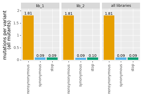
First make a plot using the default plotnine theme:

# NBVAL_IGNORE_OUTPUT

p = variants.plotNumCodonMutsByType("all", samples=None)
_ = p.draw(show=True)

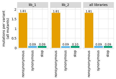
The dms_variants package defines a gray grid plotnine theme in dms_variants.plotnine_themes that gives an especially nice appearance for the plots. Here we set that theme and then re-draw the above plot:

_ = theme_set(dms_variants.plotnine_themes.theme_graygrid())

# NBVAL_IGNORE_OUTPUT

p = variants.plotNumCodonMutsByType("all", samples=None)
_ = p.draw(show=True)

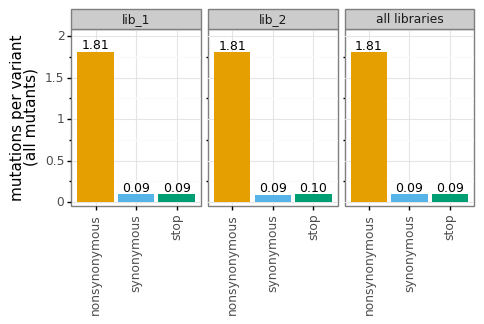
The plot looks even cleaner if we get rid of the vertical grid lines:

# NBVAL_IGNORE_OUTPUT

p = p + theme(panel_grid_major_x=element_blank())  # no vertical grid lines
_ = p.draw(show=True)

There are also lots of other themes defined by plotnine:

# NBVAL_IGNORE_OUTPUT

theme_set(theme_bw())
p = variants.plotNumCodonMutsByType("all", samples=None)
_ = p.draw(show=True)

Or more silly:

# NBVAL_IGNORE_OUTPUT

theme_set(theme_xkcd())
p = variants.plotNumCodonMutsByType(
    "all", samples=None, heightscale=1.2, widthscale=1.2
)
_ = p.draw(show=True)

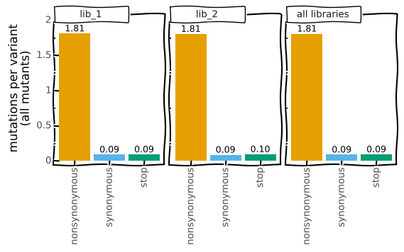
Note how the above call also used the heightscale and widthscale options (which exist for all plotting methods of a CodonVariantTable) to make the plot larger.

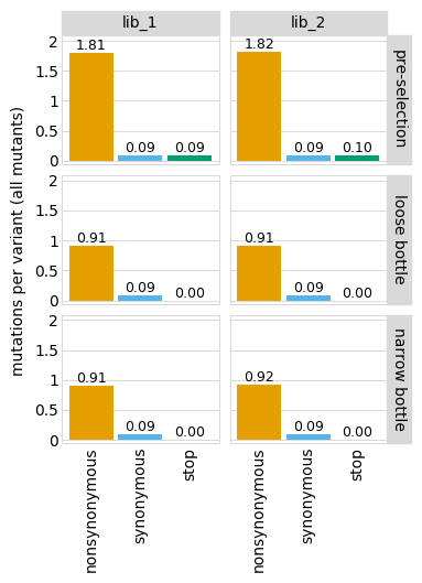
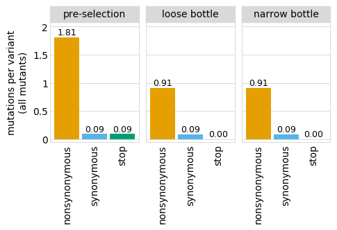
You can also set the orientation differently with orientation, and rename samples with sample_rename:

# NBVAL_IGNORE_OUTPUT

theme_set(dms_variants.plotnine_themes.theme_graygrid())  # restore gray-grid theme

p = variants.plotNumCodonMutsByType(
    "all",
    samples="all",
    orientation="v",
    heightscale=1.2,
    sample_rename={"loose_bottle": "loose bottle", "tight_bottle": "narrow bottle"},
)
p = p + theme(panel_grid_major_x=element_blank())  # no vertical grid lines
_ = p.draw(show=True)

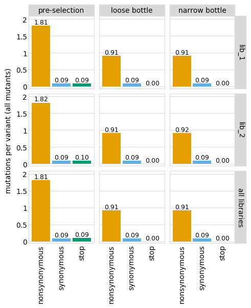
Or only show some of the facets. For instance, just show the individual libraries:

# NBVAL_IGNORE_OUTPUT

p = variants.plotNumCodonMutsByType(
    "all",
    samples="all",
    libraries=variants.libraries,
    sample_rename={"loose_bottle": "loose bottle", "tight_bottle": "narrow bottle"},
)
p = p + theme(panel_grid_major_x=element_blank())  # no vertical grid lines
_ = p.draw(show=True)

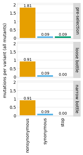
Note that if you just specify one library, by default the library name is not shown in the facet title:

# NBVAL_IGNORE_OUTPUT

p = variants.plotNumCodonMutsByType(
    "all",
    samples="all",
    libraries=["lib_1"],
    sample_rename={"loose_bottle": "loose bottle", "tight_bottle": "narrow bottle"},
)
p = p + theme(panel_grid_major_x=element_blank())  # no vertical grid lines
_ = p.draw(show=True)

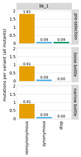
You can change this behavior by setting the one_lib_facet parameter to True:

# NBVAL_IGNORE_OUTPUT

p = variants.plotNumCodonMutsByType(
    "all",
    samples="all",
    libraries=["lib_1"],
    sample_rename={"loose_bottle": "loose bottle", "tight_bottle": "narrow bottle"},
    one_lib_facet=True,
)
p = p + theme(panel_grid_major_x=element_blank())  # no vertical grid lines
_ = p.draw(show=True)

Or only the merge of all libraries:

# NBVAL_IGNORE_OUTPUT

p = variants.plotNumCodonMutsByType(
    "all",
    samples="all",
    libraries="all_only",
    sample_rename={"loose_bottle": "loose bottle", "tight_bottle": "narrow bottle"},
    orientation="v",
)
p = p + theme(panel_grid_major_x=element_blank())  # no vertical grid lines
_ = p.draw(show=True)

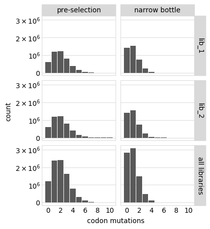
Or only show some samples:

# NBVAL_IGNORE_OUTPUT

p = variants.plotNumMutsHistogram(
    mut_type="codon",
    samples=["pre-selection", "tight_bottle"],
    orientation="v",
    sample_rename={"loose_bottle": "loose bottle", "tight_bottle": "narrow bottle"},
)
p = p + theme(panel_grid_major_x=element_blank())  # no vertical grid lines
_ = p.draw(show=True)

You can also save the plots to image files using their save method. Here we show how to do this, saving the plot as a PNG to a temporary file and then displaying that PNG:

with tempfile.NamedTemporaryFile(suffix=".png") as f:
    p.save(f.name)
    display(Image(f.name))