Libraries with secondary target genes

A CodonVariantTable is designed to handle mutations to a specific target gene. But in some cases, you might also want to include specific targets that are not point mutants of this primary target gene, but rather are entirely different genes that are spiked into the library as a control or for comparison. Because these secondary targets might not be closely related to the primary target gene, we do not want to define them simply by their mutations relative to the primary target. Rather, we handle them as different targets by adding a “targets” column in the data.

This notebook illustrates how to do this.

Setup for analysis

Import Python modules / packages:

import itertools
import random
import tempfile
import warnings

import numpy

import pandas as pd

from plotnine import *

import dms_variants.codonvarianttable
import dms_variants.plotnine_themes
import dms_variants.simulate
from dms_variants.constants import CBPALETTE, CODONS_NOSTOP

Set parameters that define the simulated data for the primary target gene. Except for that fact that we use a short gene to reduce the computational run-time of this notebook, these simulation parameters are designed to reflect what we might observe in a real Bloom lab deep mutational scanning experiment:

primary_target = "primary_target_gene"
seed = 1  # random number seed
genelength = 30  # gene length in codons
libs = ["lib_1", "lib_2"]  # distinct libraries of gene
variants_per_lib = 500 * genelength  # variants per library
avgmuts = 2.0  # average codon mutations per variant
bclen = 16  # length of nucleotide barcode for each variant
variant_error_rate = 0.005  # rate at which variant sequence mis-called
avgdepth_per_variant = 200  # average per-variant sequencing depth
lib_uniformity = 5  # uniformity of library pre-selection
noise = 0.02  # random noise in selections
bottlenecks = {  # bottlenecks from pre- to post-selection
    "tight_bottle": variants_per_lib * 5,
    "loose_bottle": variants_per_lib * 100,
}

We also define some secondary targets:

secondary_targets = [f"secondary_target_{i}" for i in range(1, 4)]

Seed random number generator for reproducible output:

random.seed(seed)
numpy.random.seed(seed)

Set pandas display options to show large chunks of Data Frames in this example:

pd.set_option("display.max_columns", 20)
pd.set_option("display.width", 500)

Hide warnings that clutter output:

warnings.simplefilter("ignore")

Set the gray grid plotnine theme defined in dms_variants.plotnine_themes as this gives a nice appearance for the plots:

theme_set(dms_variants.plotnine_themes.theme_graygrid())

Simulate library with primary and secondary variants

Simulate wildtype gene sequence:

geneseq = "".join(random.choices(CODONS_NOSTOP, k=genelength))
print(f"Wildtype gene of {genelength} codons:\n{geneseq}")

Wildtype gene of 30 codons:
AGATCCGTGATTCTGCGTGCTTACACCAACTCACGGGTGAAACGTGTAATCTTATGCAACAACGACTTACCTATCCGCAACATCCGGCTG

Generate a CodonVariantTable using simulate_CodonVariantTable function, then get the barcode-variant data frame for it. This data frame gives the variants for the primary target:

primary_bc_variant_df = dms_variants.simulate.simulate_CodonVariantTable(
    geneseq=geneseq,
    bclen=bclen,
    library_specs={
        lib: {"avgmuts": avgmuts, "nvariants": variants_per_lib} for lib in libs
    },
    seed=seed,
).barcode_variant_df

primary_bc_variant_df.head()

	library	barcode	variant_call_support	codon_substitutions	aa_substitutions	n_codon_substitutions	n_aa_substitutions
0	lib_1	AAAAAAAACGTTTTGT	1	CTG5TGG TCA11TCT	L5W	2	1
1	lib_1	AAAAAAAGGCTTATAC	5	TCA11TGC	S11C	1	1
2	lib_1	AAAAAAATCGTCCGTG	2			0	0
3	lib_1	AAAAAAGACAACACCG	5	ATC25TTC	I25F	1	1
4	lib_1	AAAAAAGATGTGGTGG	3	TCA11TTA CGG12GGT CGT15TGA ATC25GGA ATC28CGC	S11L R12G R15* I25G I28R	5	5

This data frame gives variants for the primary target, so add a column specifying that fact:

primary_bc_variant_df = primary_bc_variant_df.assign(target=primary_target)

Now add some barcodes for each secondary targets. We simulate barcodes for each secondary target and each library. Note that the secondary targets are defined genes, so we don’t add any information on substitutions for these:

existing_barcodes = set(primary_bc_variant_df["barcode"])

secondary_bc_variant_df = []
for lib, secondary_target in itertools.product(libs, secondary_targets):
    secondary_target_barcodes = dms_variants.simulate.rand_seq(
        seqlen=bclen,
        exclude=existing_barcodes,
        nseqs=random.randint(50, 100),
    )
    existing_barcodes = existing_barcodes.union(secondary_target_barcodes)
    secondary_bc_variant_df.append(
        pd.DataFrame(
            {
                "target": secondary_target,
                "barcode": secondary_target_barcodes,
                "library": lib,
                "variant_call_support": 10,
            }
        )
    )

secondary_bc_variant_df = pd.concat(secondary_bc_variant_df, ignore_index=True)

secondary_bc_variant_df.head()

	target	barcode	library	variant_call_support
0	secondary_target_1	TCCTGTACGATATCCC	lib_1	10
1	secondary_target_1	GGGTGTGGCGTTTCCT	lib_1	10
2	secondary_target_1	TAGCCTCTATTGCCTT	lib_1	10
3	secondary_target_1	CGGAGACGTCACGGCG	lib_1	10
4	secondary_target_1	GGGGACAATTATCCCT	lib_1	10

Concatenate the data frame for the primary target (which has mutants) with that for the secondary targets. Because there are no mutations for the secondary targets, fill that information is as empty strings (for substitution columns) or 0 (for number of mutations). This data frame below ends the simulation of the library, and represents the type of information you would typically have at the outset of an experiment:

bc_variant_df = pd.concat(
    [primary_bc_variant_df, secondary_bc_variant_df], sort=False
).assign(
    codon_substitutions=lambda x: x["codon_substitutions"].fillna(""),
    aa_substitutions=lambda x: x["aa_substitutions"].fillna(""),
    n_codon_substitutions=lambda x: x["n_codon_substitutions"].fillna(0).astype(int),
    n_aa_substitutions=lambda x: x["n_aa_substitutions"].fillna(0).astype(int),
)

bc_variant_df

	library	barcode	variant_call_support	codon_substitutions	aa_substitutions	n_codon_substitutions	n_aa_substitutions	target
0	lib_1	AAAAAAAACGTTTTGT	1	CTG5TGG TCA11TCT	L5W	2	1	primary_target_gene
1	lib_1	AAAAAAAGGCTTATAC	5	TCA11TGC	S11C	1	1	primary_target_gene
2	lib_1	AAAAAAATCGTCCGTG	2			0	0	primary_target_gene
3	lib_1	AAAAAAGACAACACCG	5	ATC25TTC	I25F	1	1	primary_target_gene
4	lib_1	AAAAAAGATGTGGTGG	3	TCA11TTA CGG12GGT CGT15TGA ATC25GGA ATC28CGC	S11L R12G R15* I25G I28R	5	5	primary_target_gene
...	...	...	...	...	...	...	...	...
429	lib_2	GCGGCCTGGAGTTGAA	10			0	0	secondary_target_3
430	lib_2	TGATCACTACGTCCTT	10			0	0	secondary_target_3
431	lib_2	TTTAGGAATCTCCCGT	10			0	0	secondary_target_3
432	lib_2	TGTGCTTAGAGCACCG	10			0	0	secondary_target_3
433	lib_2	TTCTTACTGAAGTTCC	10			0	0	secondary_target_3

30434 rows × 8 columns

Now create the CodonVariantTable. Note how we specify the primary_target option to the name of that target; this is required when using multiple targets:

with tempfile.NamedTemporaryFile() as f:
    bc_variant_df.to_csv(f.name, index=False)
    f.flush()
    variants = dms_variants.codonvarianttable.CodonVariantTable(
        barcode_variant_file=f.name,
        geneseq=geneseq,
        substitutions_are_codon=True,
        substitutions_col="codon_substitutions",
        primary_target=primary_target,
    )

We can get basic information about the CodonVariantTable, such as the sites, wildtype codons, and wildtype amino acids. Below we do this for the first few sites. Note that all of this information is for the primary target:

variants.sites[:5]

[1, 2, 3, 4, 5]

list(variants.codons[r] for r in variants.sites[:5])

['AGA', 'TCC', 'GTG', 'ATT', 'CTG']

list(variants.aas[r] for r in variants.sites[:5])

['R', 'S', 'V', 'I', 'L']

The different libraries in the table:

variants.libraries

['lib_1', 'lib_2']

Here is the data frame that contains all of the information on the barcoded variants. Note that the list of substitutions for the secondary targets just repeat the target name (so you are not confused with thinking mutations are actually enumerated in these secondary targets):

variants.barcode_variant_df

	target	library	barcode	variant_call_support	codon_substitutions	aa_substitutions	n_codon_substitutions	n_aa_substitutions
0	primary_target_gene	lib_1	AAAAAAAACGTTTTGT	1	CTG5TGG TCA11TCT	L5W	2	1
1	primary_target_gene	lib_1	AAAAAAAGGCTTATAC	5	TCA11TGC	S11C	1	1
2	primary_target_gene	lib_1	AAAAAAATCGTCCGTG	2			0	0
3	primary_target_gene	lib_1	AAAAAAGACAACACCG	5	ATC25TTC	I25F	1	1
4	primary_target_gene	lib_1	AAAAAAGATGTGGTGG	3	TCA11TTA CGG12GGT CGT15TGA ATC25GGA ATC28CGC	S11L R12G R15* I25G I28R	5	5
...	...	...	...	...	...	...	...	...
30429	secondary_target_3	lib_2	TGTGCTTAGAGCACCG	10	secondary_target_3	secondary_target_3	0	0
30430	secondary_target_3	lib_2	TTCCGACACGTTGACC	10	secondary_target_3	secondary_target_3	0	0
30431	secondary_target_3	lib_2	TTCTATTACGCTGGGG	10	secondary_target_3	secondary_target_3	0	0
30432	secondary_target_3	lib_2	TTCTTACTGAAGTTCC	10	secondary_target_3	secondary_target_3	0	0
30433	secondary_target_3	lib_2	TTTAGGAATCTCCCGT	10	secondary_target_3	secondary_target_3	0	0

30434 rows × 8 columns

Analyze library composition

A CodonVariantTable has methods for summarizing and plotting properties of the barcoded variants. These methods can be used to analyze the barcoded variants themselves, or to analyze the frequency (or counts) of variants in the library in samples that have undergone some type of selection.

We have not yet added counts of the variants in any specific samples, so we just analyze the composition of the variant library itself. This is done by setting samples=None in the method calls below.

Number of variants in each library:

variants.n_variants_df(samples=None)

	target	library	sample	count
0	primary_target_gene	lib_1	barcoded variants	15000
1	primary_target_gene	lib_2	barcoded variants	15000
2	primary_target_gene	all libraries	barcoded variants	30000
3	secondary_target_1	lib_1	barcoded variants	52
4	secondary_target_1	lib_2	barcoded variants	82
5	secondary_target_1	all libraries	barcoded variants	134
6	secondary_target_2	lib_1	barcoded variants	89
7	secondary_target_2	lib_2	barcoded variants	69
8	secondary_target_2	all libraries	barcoded variants	158
9	secondary_target_3	lib_1	barcoded variants	87
10	secondary_target_3	lib_2	barcoded variants	55
11	secondary_target_3	all libraries	barcoded variants	142

We can also get this information for just the primary target:

variants.n_variants_df(samples=None, primary_target_only=True)

	library	sample	count
0	lib_1	barcoded variants	15000
1	lib_2	barcoded variants	15000
2	all libraries	barcoded variants	30000

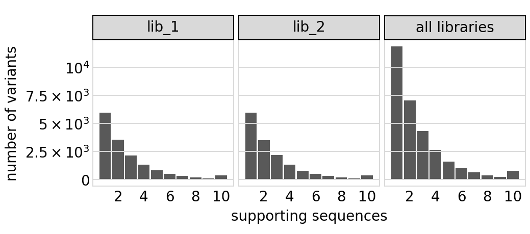
Plot distribution of variant call supports, grouping together all variants with support \(\ge 8\):

# NBVAL_IGNORE_OUTPUT

p = variants.plotVariantSupportHistogram(max_support=10)
p = p + theme(panel_grid_major_x=element_blank())  # no vertical grid lines
_ = p.draw(show=True)

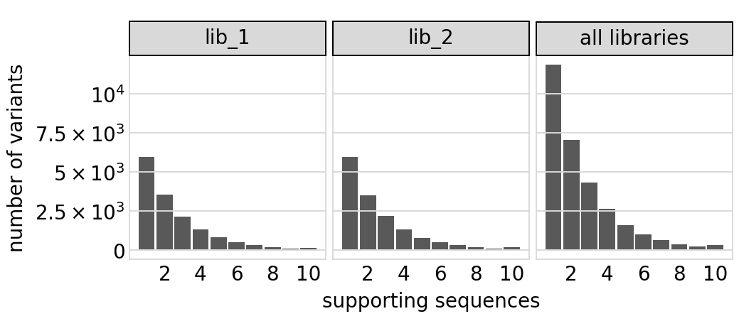
Same plot for only the primary target:

# NBVAL_IGNORE_OUTPUT

p = variants.plotVariantSupportHistogram(max_support=10, primary_target_only=True)
p = p + theme(panel_grid_major_x=element_blank())  # no vertical grid lines
_ = p.draw(show=True)

The set of valid barcodes for each library:

for lib in libs:
    print(f"First few barcodes for library {lib}:")
    print(sorted(variants.valid_barcodes(lib))[:3])

First few barcodes for library lib_1:
['AAAAAAAACGTTTTGT', 'AAAAAAAGGCTTATAC', 'AAAAAAATCGTCCGTG']
First few barcodes for library lib_2:
['AAAAAACCCAGACTTA', 'AAAAAACCGGCGGCAG', 'AAAAAATCTACTGCGT']

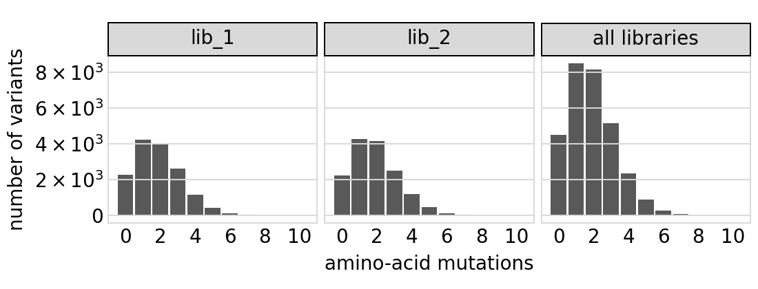
Plot the number of amino-acid mutations per variant. Note that this plot is only for the primary target:

# NBVAL_IGNORE_OUTPUT

p = variants.plotNumMutsHistogram("aa", samples=None)
p = p + theme(panel_grid_major_x=element_blank())  # no vertical grid lines
_ = p.draw(show=True)

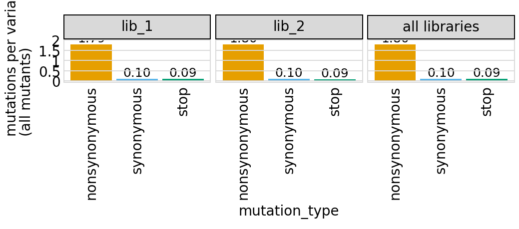
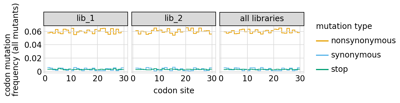
Average number of codon mutations per variant of each type of mutation. We make these plots for: 1. Just single-mutant and wildtype variants 2. For all variants

Again, these are only for the primary target, since mutations are only defined for that target:

# NBVAL_IGNORE_OUTPUT

for mut_type in ["single", "all"]:
    p = variants.plotNumCodonMutsByType(mut_type, samples=None)
    p = p + theme(panel_grid_major_x=element_blank())  # no vertical grid lines
    _ = p.draw(show=True)

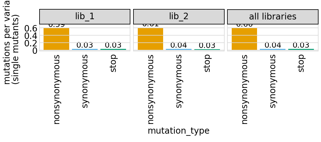
Here are the numerical data in the plots above:

variants.numCodonMutsByType("single", samples=None).round(3)

	library	sample	mutation_type	num_muts_count	count	number
0	lib_1	barcoded variants	nonsynonymous	3615	6112	0.591
1	lib_1	barcoded variants	synonymous	194	6112	0.032
2	lib_1	barcoded variants	stop	211	6112	0.035
3	lib_2	barcoded variants	nonsynonymous	3716	6114	0.608
4	lib_2	barcoded variants	synonymous	235	6114	0.038
5	lib_2	barcoded variants	stop	179	6114	0.029
6	all libraries	barcoded variants	nonsynonymous	7331	12226	0.600
7	all libraries	barcoded variants	synonymous	429	12226	0.035
8	all libraries	barcoded variants	stop	390	12226	0.032

variants.numCodonMutsByType("all", samples=None).round(3)

	library	sample	mutation_type	num_muts_count	count	number
0	lib_1	barcoded variants	nonsynonymous	26916	15000	1.794
1	lib_1	barcoded variants	synonymous	1510	15000	0.101
2	lib_1	barcoded variants	stop	1424	15000	0.095
3	lib_2	barcoded variants	nonsynonymous	26960	15000	1.797
4	lib_2	barcoded variants	synonymous	1498	15000	0.100
5	lib_2	barcoded variants	stop	1371	15000	0.091
6	all libraries	barcoded variants	nonsynonymous	53876	30000	1.796
7	all libraries	barcoded variants	synonymous	3008	30000	0.100
8	all libraries	barcoded variants	stop	2795	30000	0.093

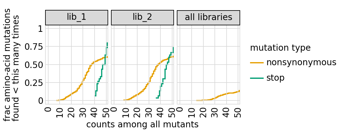
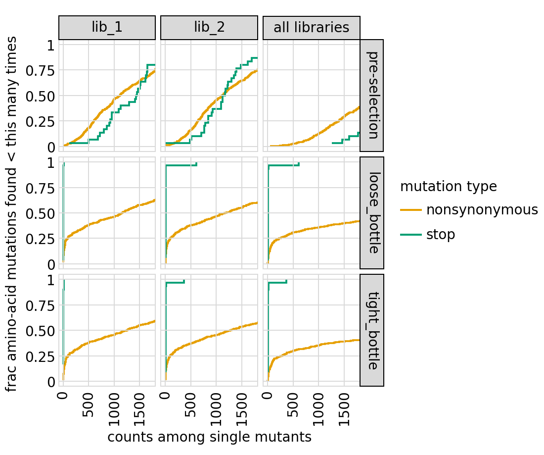
Examine how well amino-acid mutations to the primary target are sampled in the library by looking at the fraction of mutations seen <= some number of times. Here we do that for amino-acid mutations, making separate plots for single mutants and all mutants:

# NBVAL_IGNORE_OUTPUT

for variant_type in ["single", "all"]:
    p = variants.plotCumulMutCoverage(variant_type, mut_type="aa", samples=None)
    _ = p.draw(show=True)

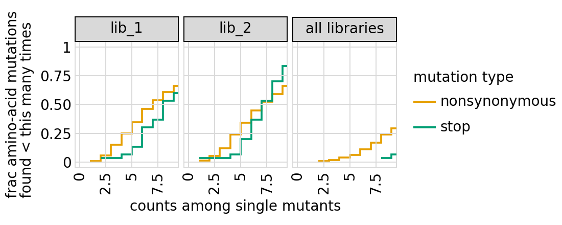
We can also get the numerical information plotted above (here for single mutants only):

variants.mutCounts("single", "aa", samples=None).head(n=5)

	library	sample	mutation	count	mutation_type	site
0	lib_1	barcoded variants	V16L	25	nonsynonymous	16
1	lib_1	barcoded variants	C19R	21	nonsynonymous	19
2	lib_1	barcoded variants	R12S	21	nonsynonymous	12
3	lib_1	barcoded variants	R26L	21	nonsynonymous	26
4	lib_1	barcoded variants	S11R	21	nonsynonymous	11

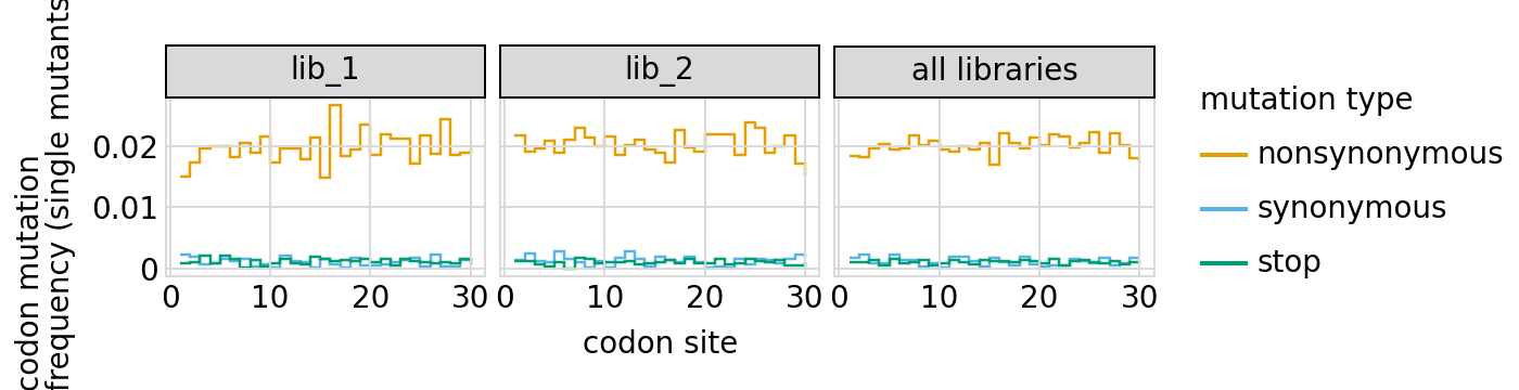
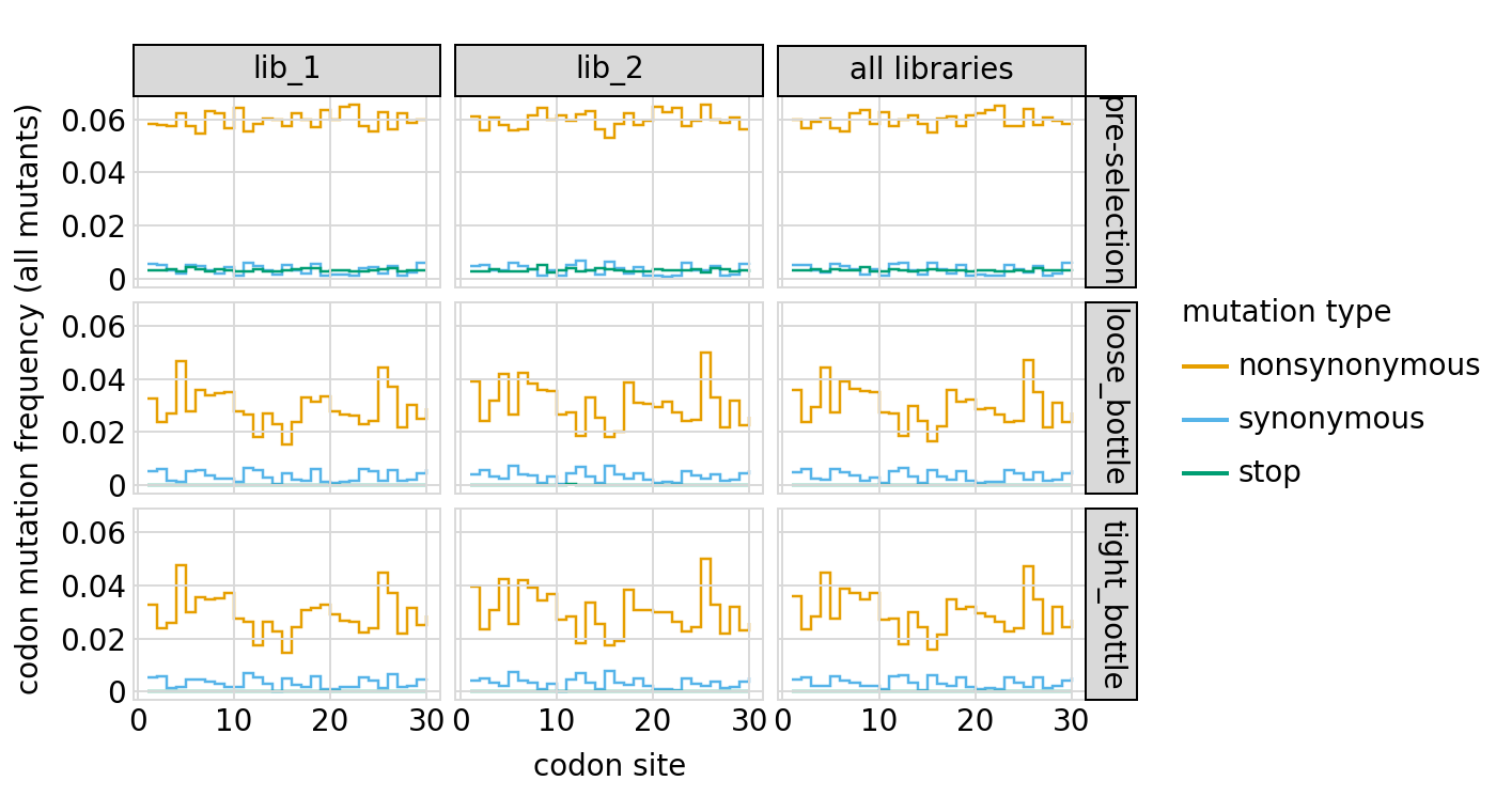
Here are the frequencies of mutations along the primary target gene, looking both at single mutants and all mutants:

# NBVAL_IGNORE_OUTPUT

for variant_type in ["single", "all"]:
    p = variants.plotMutFreqs(variant_type, "codon", samples=None)
    _ = p.draw(show=True)

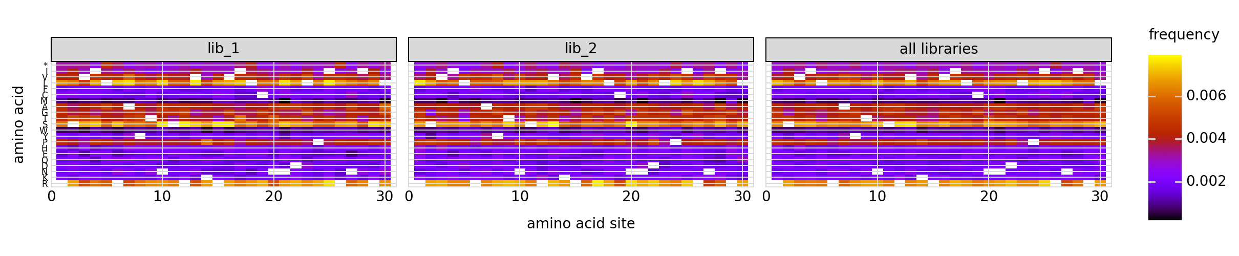
We can also look at mutation frequencies in the primary target gene a heat-map form:

# NBVAL_IGNORE_OUTPUT

p = variants.plotMutHeatmap("all", "aa", samples=None)
_ = p.draw(show=True)

Simulate counts for samples

An experiment involves subjecting the library to different selections and looking at how the frequencies of the variants changes by using sequencing to count the barcodes in each condition.

Here, we simulate an experiment by simulating variant counts for samples that have undergone various selections.

For these simulations, we first need to define a “phenotype” for each variant. The phenotype represents how much the frequency of the variant is expected to increase or decrease after selection.

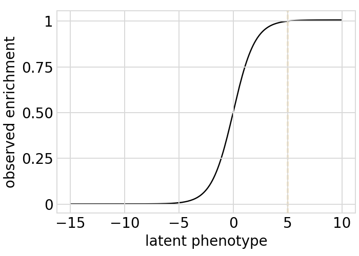
Define phenotype function

First, we define a “phenotype” function. We will do this using a SigmoidPhenotypeSimulator, which follow the “global epistasis” concepts of Otwinoski et al and Sailer and Harms to define the phenotype in two steps: an underlying latent phenotype that mutations affect additively, and then an observed phenotype that is a non-linear function of the latent phenotype. The variants are then simulated according to their observed enrichments, which are the exponentials of the observed phenotypes.

First, we initialize the simulator:

phenosimulator = dms_variants.simulate.SigmoidPhenotypeSimulator(geneseq, seed=seed)

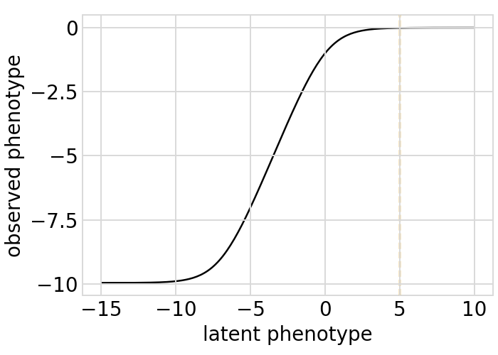
Plot the simulated relationship of the latent phenotype with the observed enrichment and phenotype, with a dashed vertical line indicating the wildtype latent phenotype:

# NBVAL_IGNORE_OUTPUT

for value in ["enrichment", "phenotype"]:
    p = phenosimulator.plotLatentVsObserved(value)
    _ = p.draw(show=True)

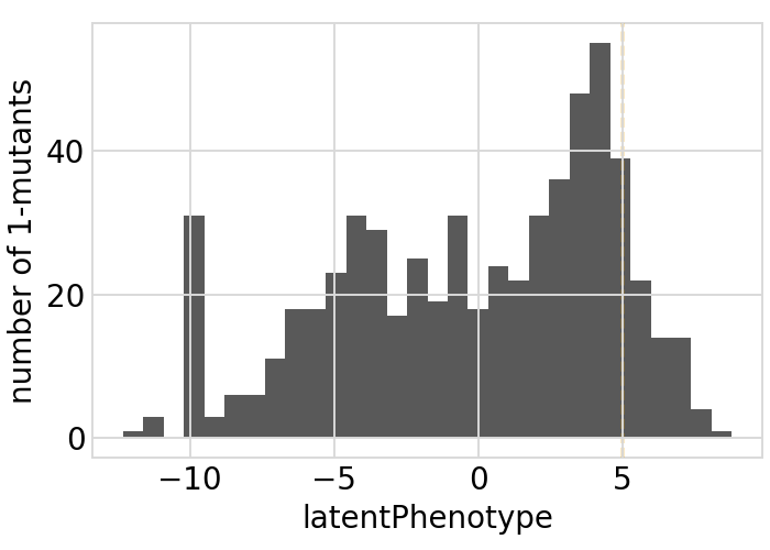
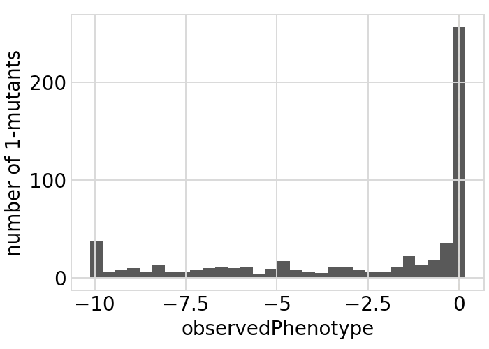
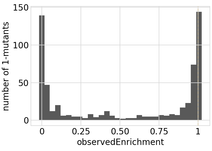
Plot the latent phenotype, observed phenotype, and observed enrichment of all single amino-acid mutants, with a dashed vertical line indicating the wildtype:

# NBVAL_IGNORE_OUTPUT

for value in ["latentPhenotype", "observedPhenotype", "observedEnrichment"]:
    p = phenosimulator.plotMutsHistogram(value)
    _ = p.draw(show=True)

Phenotypes for secondary targets

We also specify phenotypes as observed enrichments for the secondary targets:

secondary_target_phenotypes = {
    secondary_target: round(random.uniform(0.2, 2), 3)
    for secondary_target in secondary_targets
}

# display the observed enrichments for the secondary targets
pd.Series(secondary_target_phenotypes).rename("observed_enrichment").to_frame()

	observed_enrichment
secondary_target_1	0.883
secondary_target_2	1.211
secondary_target_3	1.789

Simulate variant counts

Now we use simulateSampleCounts to simulate counts of variants when selection on each variant is proportional to its observed enrichment. In these simulations, we can fine-tune the simulations to reflect real experiments, such as by setting the error-rate in variant calling, bottlenecks when going from the pre- to post-selection samples, and non-uniformity in library composition.

Here we simulate using several bottlenecks in the library going from the pre- to post-selection samples, since in real experiments this seems to be the biggest source of noise / error:

counts = dms_variants.simulate.simulateSampleCounts(
    variants=variants,
    phenotype_func=phenosimulator.observedEnrichment,
    variant_error_rate=variant_error_rate,
    pre_sample={
        "total_count": variants_per_lib * numpy.random.poisson(avgdepth_per_variant),
        "uniformity": lib_uniformity,
    },
    pre_sample_name="pre-selection",
    post_samples={
        name: {
            "noise": noise,
            "total_count": variants_per_lib
            * numpy.random.poisson(avgdepth_per_variant),
            "bottleneck": bottle,
        }
        for name, bottle in bottlenecks.items()
    },
    seed=seed,
    secondary_target_phenotypes=secondary_target_phenotypes,
)

Data frame with the simulated counts:

counts.head(6)

	library	barcode	sample	count
0	lib_1	AAAAAAAACGTTTTGT	pre-selection	317
1	lib_1	AAAAAAAGGCTTATAC	pre-selection	133
2	lib_1	AAAAAAATCGTCCGTG	pre-selection	127
3	lib_1	AAAAAAGACAACACCG	pre-selection	97
4	lib_1	AAAAAAGATGTGGTGG	pre-selection	324
5	lib_1	AAAAAAGTCATACTCG	pre-selection	118

Add counts to variant table

Now add the simulated counts for each library / sample to the CodonVariantTable:

variants.add_sample_counts_df(counts)

Confirm that we have added the expected number of counts per library / sample:

# NBVAL_IGNORE_OUTPUT

variants.n_variants_df(libraries="all_only")

	target	library	sample	count
0	primary_target_gene	all libraries	pre-selection	5439967
1	primary_target_gene	all libraries	loose_bottle	5366820
2	primary_target_gene	all libraries	tight_bottle	5916597
3	secondary_target_1	all libraries	pre-selection	23756
4	secondary_target_1	all libraries	loose_bottle	54373
5	secondary_target_1	all libraries	tight_bottle	57359
6	secondary_target_2	all libraries	pre-selection	29184
7	secondary_target_2	all libraries	loose_bottle	92595
8	secondary_target_2	all libraries	tight_bottle	98230
9	secondary_target_3	all libraries	pre-selection	27093
10	secondary_target_3	all libraries	loose_bottle	126212
11	secondary_target_3	all libraries	tight_bottle	137814

Look only for primary target:

# NBVAL_IGNORE_OUTPUT

variants.n_variants_df(primary_target_only=True)

	library	sample	count
0	lib_1	pre-selection	2719365
1	lib_1	loose_bottle	2674231
2	lib_1	tight_bottle	2949688
3	lib_2	pre-selection	2720602
4	lib_2	loose_bottle	2692589
5	lib_2	tight_bottle	2966909
6	all libraries	pre-selection	5439967
7	all libraries	loose_bottle	5366820
8	all libraries	tight_bottle	5916597

Analyze sample variant counts

A CodonVariantTable has methods for summarizing and plotting the variant counts for different samples. These methods are mostly the same as we used above to analyze the variant composition of the libraries themselves, but now we set samples to the samples that we want to analyze (typically 'all'). Therefore, rather than each variant always counting once, each variant is counted in each sample in proportion to how many counts it has.

In the rawest form, we can directly access a data frame giving the counts of each variant in each sample:

# NBVAL_IGNORE_OUTPUT

variants.variant_count_df

	target	library	sample	barcode	count	variant_call_support	codon_substitutions	aa_substitutions	n_codon_substitutions	n_aa_substitutions
0	primary_target_gene	lib_1	pre-selection	AACCCGTTCACCACCA	692	2	ATC17CGA CGG29TGC	I17R R29C	2	2
1	primary_target_gene	lib_1	pre-selection	ACTACGGACGATTATT	633	1	GCT7TCT AAA14GAT AAC20CGA	A7S K14D N20R	3	3
2	primary_target_gene	lib_1	pre-selection	GGACTATCTCAGTATG	615	2			0	0
3	primary_target_gene	lib_1	pre-selection	CCAGAAAACCCACCAA	614	7	TTA18CTC		1	0
4	primary_target_gene	lib_1	pre-selection	ACGGCCTAAACTCACA	611	3	CGT6GTA GAC22CAC	R6V D22H	2	2
...	...	...	...	...	...	...	...	...	...	...
91297	secondary_target_3	lib_2	tight_bottle	CAACCTAATTGGGATC	187	10	secondary_target_3	secondary_target_3	0	0
91298	secondary_target_3	lib_2	tight_bottle	TGGGCACGATGCAATA	186	10	secondary_target_3	secondary_target_3	0	0
91299	secondary_target_3	lib_2	tight_bottle	ACGAGTACCCCACTTC	182	10	secondary_target_3	secondary_target_3	0	0
91300	secondary_target_3	lib_2	tight_bottle	TATATCGGCGTGAAGA	176	10	secondary_target_3	secondary_target_3	0	0
91301	secondary_target_3	lib_2	tight_bottle	CAGTGGTAATTAAACG	0	10	secondary_target_3	secondary_target_3	0	0

91302 rows × 10 columns

Get the average number of counts per variant:

# NBVAL_IGNORE_OUTPUT

variants.avgCountsPerVariant().round(1)

	target	library	sample	avg_counts_per_variant
0	primary_target_gene	lib_1	pre-selection	181.3
1	primary_target_gene	lib_1	loose_bottle	178.3
2	primary_target_gene	lib_1	tight_bottle	196.6
3	primary_target_gene	lib_2	pre-selection	181.4
4	primary_target_gene	lib_2	loose_bottle	179.5
5	primary_target_gene	lib_2	tight_bottle	197.8
6	primary_target_gene	all libraries	pre-selection	181.3
7	primary_target_gene	all libraries	loose_bottle	178.9
8	primary_target_gene	all libraries	tight_bottle	197.2
9	secondary_target_1	lib_1	pre-selection	166.1
10	secondary_target_1	lib_1	loose_bottle	378.2
11	secondary_target_1	lib_1	tight_bottle	401.7
12	secondary_target_1	lib_2	pre-selection	184.4
13	secondary_target_1	lib_2	loose_bottle	423.2
14	secondary_target_1	lib_2	tight_bottle	444.8
15	secondary_target_1	all libraries	pre-selection	177.3
16	secondary_target_1	all libraries	loose_bottle	405.8
17	secondary_target_1	all libraries	tight_bottle	428.1
18	secondary_target_2	lib_1	pre-selection	173.2
19	secondary_target_2	lib_1	loose_bottle	556.6
20	secondary_target_2	lib_1	tight_bottle	611.9
21	secondary_target_2	lib_2	pre-selection	199.5
22	secondary_target_2	lib_2	loose_bottle	624.0
23	secondary_target_2	lib_2	tight_bottle	634.3
24	secondary_target_2	all libraries	pre-selection	184.7
25	secondary_target_2	all libraries	loose_bottle	586.0
26	secondary_target_2	all libraries	tight_bottle	621.7
27	secondary_target_3	lib_1	pre-selection	190.6
28	secondary_target_3	lib_1	loose_bottle	880.0
29	secondary_target_3	lib_1	tight_bottle	919.1
30	secondary_target_3	lib_2	pre-selection	191.1
31	secondary_target_3	lib_2	loose_bottle	902.7
32	secondary_target_3	lib_2	tight_bottle	1051.8
33	secondary_target_3	all libraries	pre-selection	190.8
34	secondary_target_3	all libraries	loose_bottle	888.8
35	secondary_target_3	all libraries	tight_bottle	970.5

Above the counts are grouped by target. To not group by target:

variants.avgCountsPerVariant(by_target=False).round(1)

	library	sample	avg_counts_per_variant
0	lib_1	pre-selection	181.2
1	lib_1	loose_bottle	185.2
2	lib_1	tight_bottle	203.9
3	lib_2	pre-selection	181.5
4	lib_2	loose_bottle	185.5
5	lib_2	tight_bottle	204.2
6	all libraries	pre-selection	181.4
7	all libraries	loose_bottle	185.3
8	all libraries	tight_bottle	204.0

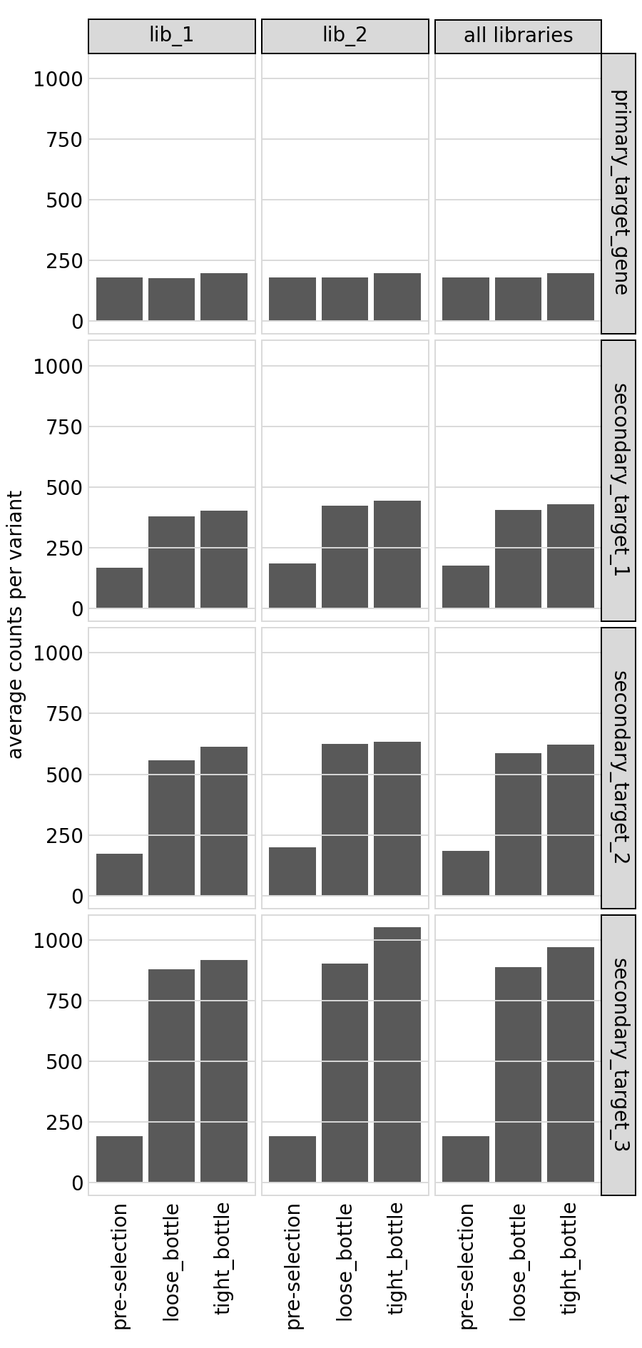
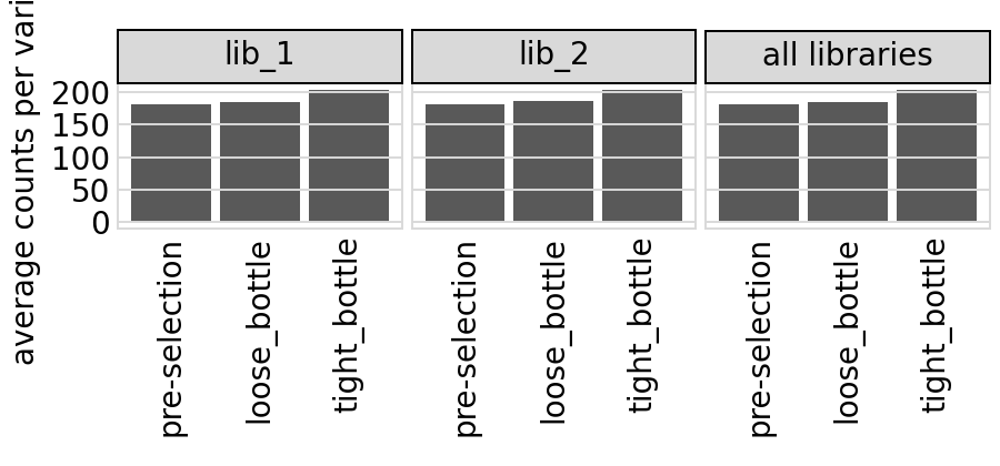
We also plot the average counts per variant:

# NBVAL_IGNORE_OUTPUT

p = variants.plotAvgCountsPerVariant(heightscale=1.5, orientation="h")
p = p + theme(panel_grid_major_x=element_blank())  # no vertical grid lines
_ = p.draw(show=True)

Here is the same plot not faceted by target:

# NBVAL_IGNORE_OUTPUT

p = variants.plotAvgCountsPerVariant(orientation="h", by_target=False)
p = p + theme(panel_grid_major_x=element_blank())  # no vertical grid lines
_ = p.draw(show=True)

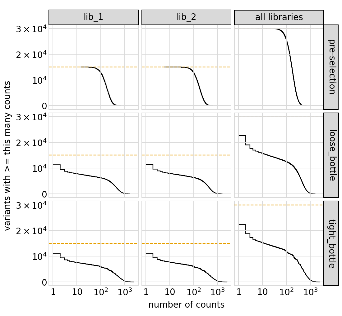
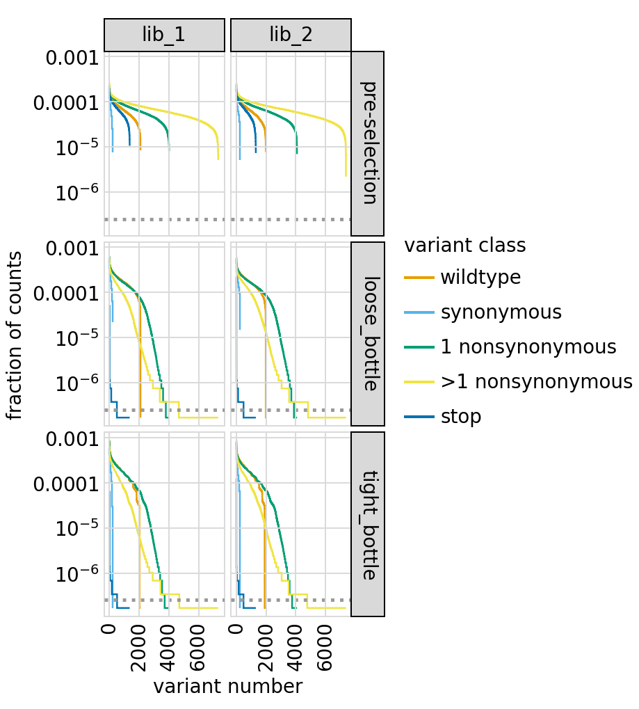
Plot the number of counts for each variant in each sample. The horizontal dashed line shows the total number of variants. The plot shows that all variants are well-sampled in the pre-selection libraries, but that post- selection some variants are sampled more or less. This is expected since selection will decrease and increase the frequency of variants. By default, this plot shows only the primary target:

# NBVAL_IGNORE_OUTPUT

p = variants.plotCumulVariantCounts()
_ = p.draw(show=True)

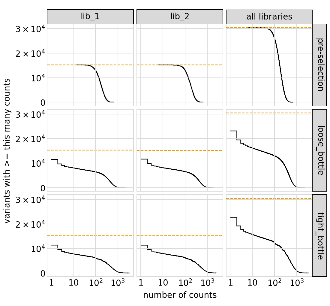
Similar plot showing all targets:

# NBVAL_IGNORE_OUTPUT

p = variants.plotCumulVariantCounts(primary_target_only=False)
_ = p.draw(show=True)

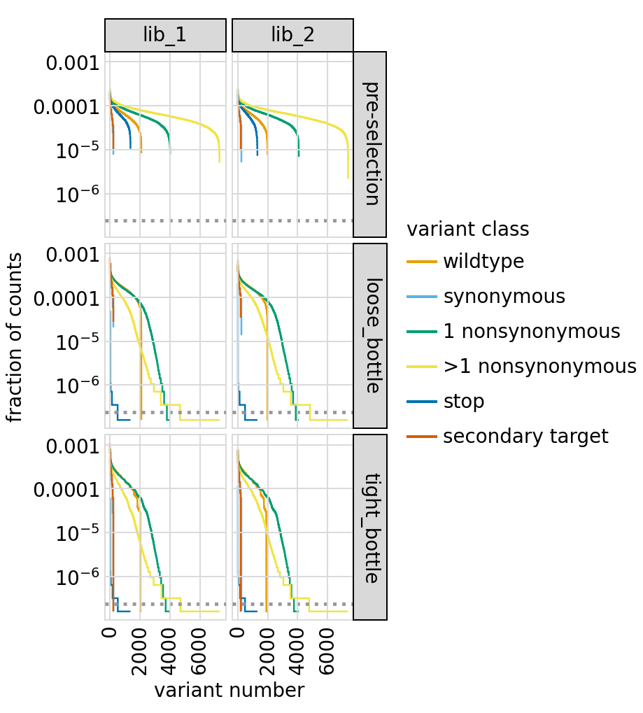
Number of counts per variant:

# NBVAL_IGNORE_OUTPUT

p = variants.plotCountsPerVariant(libraries=variants.libraries, by_variant_class=True)
_ = p.draw(show=True)

Similar plot only for primary targets:

# NBVAL_IGNORE_OUTPUT

p = variants.plotCountsPerVariant(
    libraries=variants.libraries, by_variant_class=True, primary_target_only=True
)

_ = p.draw(show=True)

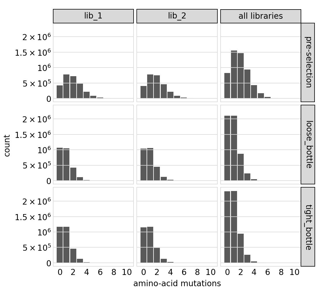
Distribution of the number of amino-acid mutations per variant in each sample. This is only for the primary target. As expected, mutations go down after selection:

# NBVAL_IGNORE_OUTPUT

p = variants.plotNumMutsHistogram(mut_type="aa")
p = p + theme(panel_grid_major_x=element_blank())  # no vertical grid lines
_ = p.draw(show=True)

Average number of mutations of each type per variant among just single mutants (and wildtype) and among all variants, again only for primary target:

# NBVAL_IGNORE_OUTPUT

for variant_type in ["single", "all"]:
    p = variants.plotNumCodonMutsByType(variant_type)
    p = p + theme(panel_grid_major_x=element_blank())  # no vertical grid lines
    _ = p.draw(show=True)

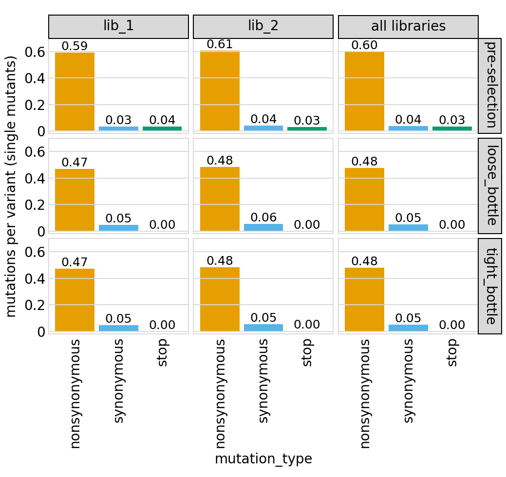
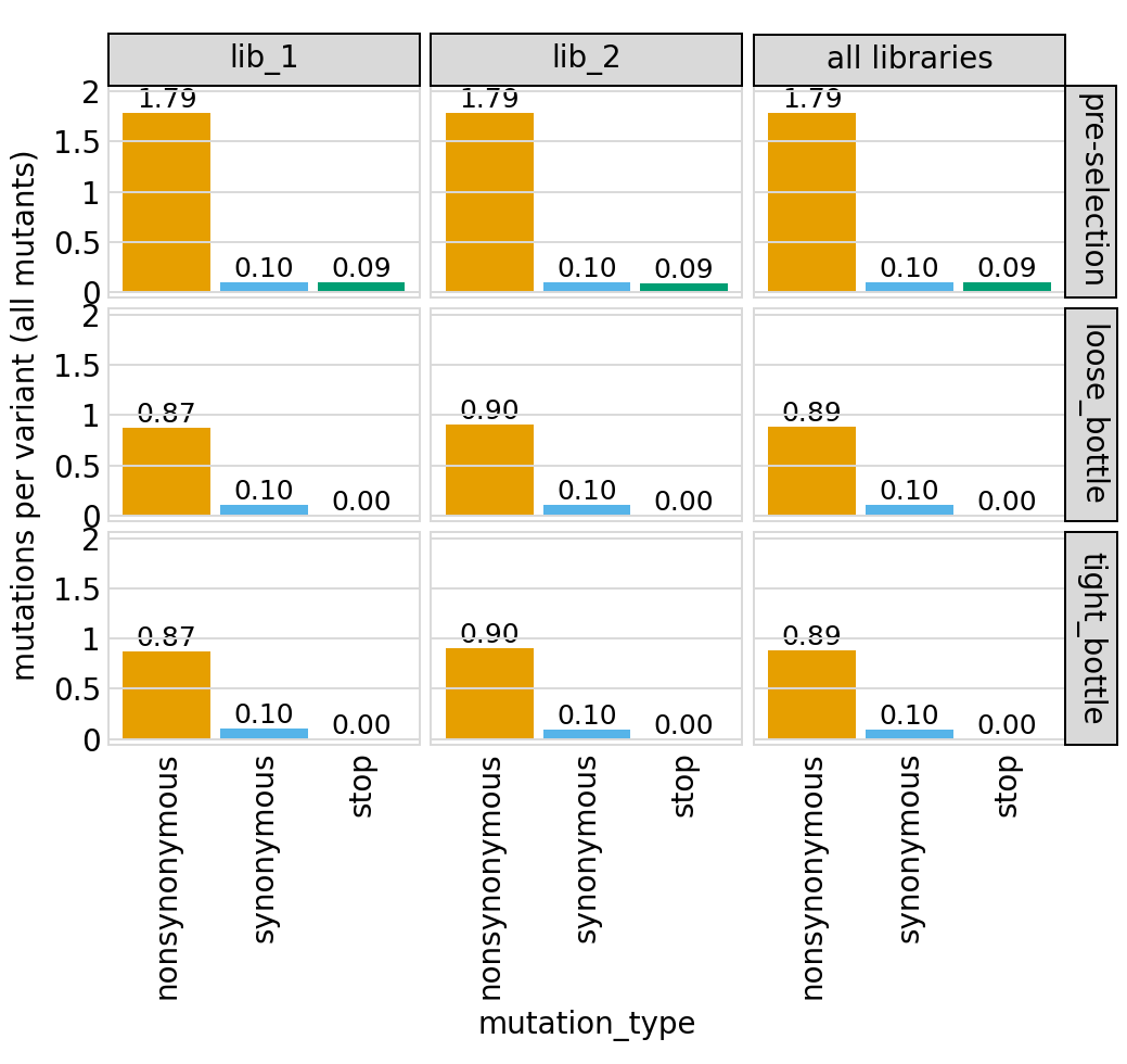
Here are the numerical data plotted above (just for the individual libraries and all mutations):

# NBVAL_IGNORE_OUTPUT

variants.numCodonMutsByType(variant_type="all", libraries=libs).round(3)

	library	sample	mutation_type	num_muts_count	count	number
0	lib_1	pre-selection	nonsynonymous	4864651	2719365	1.789
1	lib_1	pre-selection	synonymous	275311	2719365	0.101
2	lib_1	pre-selection	stop	257132	2719365	0.095
3	lib_1	loose_bottle	nonsynonymous	2330462	2674231	0.871
4	lib_1	loose_bottle	synonymous	270348	2674231	0.101
5	lib_1	loose_bottle	stop	809	2674231	0.000
6	lib_1	tight_bottle	nonsynonymous	2574335	2949688	0.873
7	lib_1	tight_bottle	synonymous	289539	2949688	0.098
8	lib_1	tight_bottle	stop	948	2949688	0.000
9	lib_2	pre-selection	nonsynonymous	4872431	2720602	1.791
10	lib_2	pre-selection	synonymous	279586	2720602	0.103
11	lib_2	pre-selection	stop	249866	2720602	0.092
12	lib_2	loose_bottle	nonsynonymous	2433719	2692589	0.904
13	lib_2	loose_bottle	synonymous	271738	2692589	0.101
14	lib_2	loose_bottle	stop	1253	2692589	0.000
15	lib_2	tight_bottle	nonsynonymous	2669151	2966909	0.900
16	lib_2	tight_bottle	synonymous	288678	2966909	0.097
17	lib_2	tight_bottle	stop	1060	2966909	0.000

Here are mutation frequencies as a function of primary sequence among all variants of the primary target:

# NBVAL_IGNORE_OUTPUT

p = variants.plotMutFreqs(variant_type="all", mut_type="codon")
_ = p.draw(show=True)

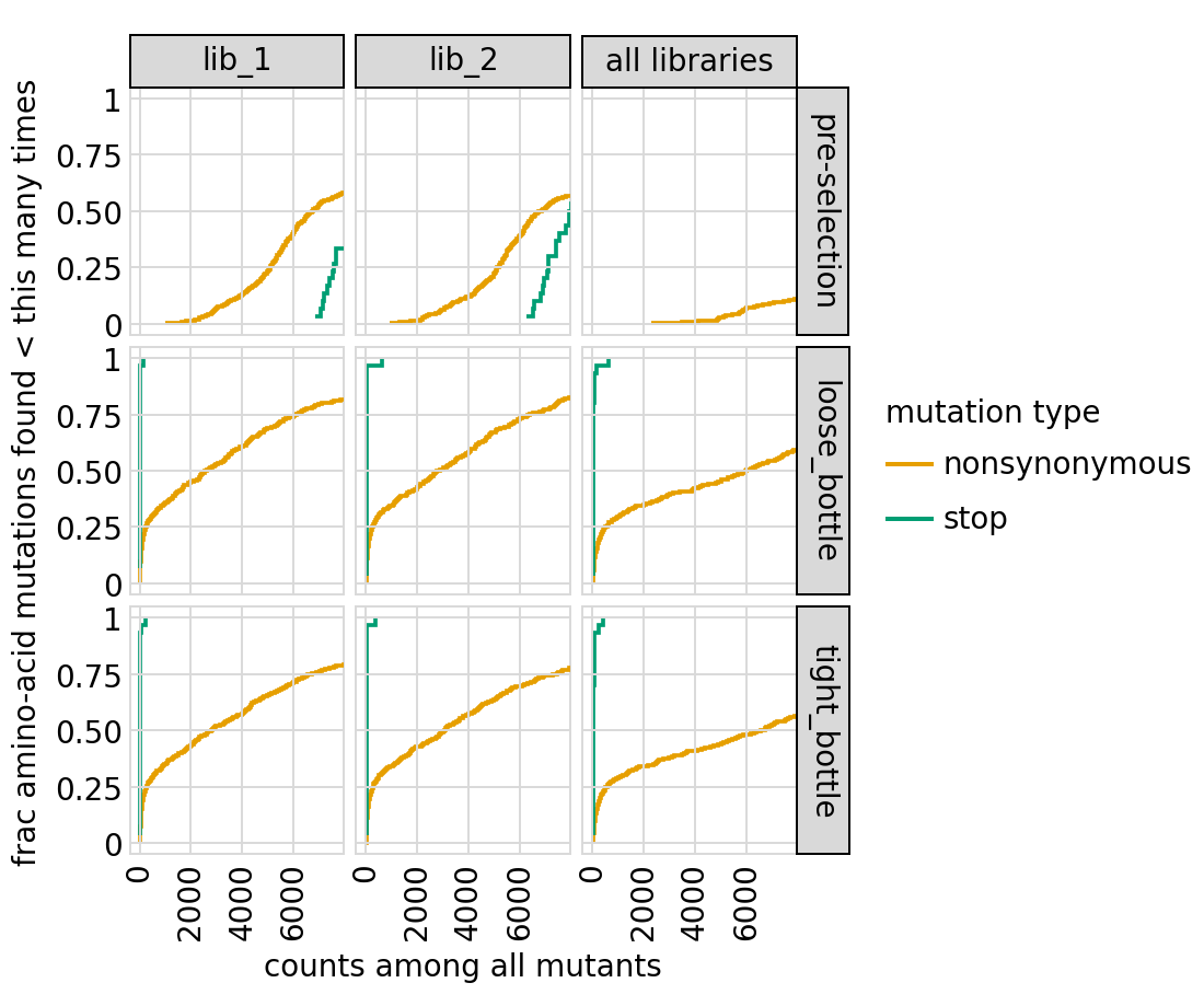
Plot how thoroughly amino-acid mutations are sampled, doing this separately among all variants and single-mutant variants for the primary target. The plots below show that the stop mutations are sampled very poorly post-selection because they are eliminated during selection:

# NBVAL_IGNORE_OUTPUT

for variant_type in ["single", "all"]:
    p = variants.plotCumulMutCoverage(variant_type=variant_type, mut_type="aa")
    _ = p.draw(show=True)

Functional scores for variants

The CodonVariantTable.func_scores method calculates a functional score for each variant based on its change in frequency from pre- to post-selection.

To calculate these scores, we need to pair each post-selection sample with a pre-selection one. In this case, the pre-selection sample is named ‘pre-selection’ for all post-selection samples:

func_scores = variants.func_scores("pre-selection", libraries=libs)

The resulting data frame has a functional score (and its variance) for each barcoded variant:

# NBVAL_IGNORE_OUTPUT

func_scores.round(3)

	target	library	pre_sample	post_sample	barcode	func_score	func_score_var	pre_count	post_count	pre_count_wt	post_count_wt	pseudocount	codon_substitutions	n_codon_substitutions	aa_substitutions	n_aa_substitutions
0	primary_target_gene	lib_1	pre-selection	loose_bottle	AACCCGTTCACCACCA	-1.060	0.005	692	847	381697	973820	0.5	ATC17CGA CGG29TGC	2	I17R R29C	2
1	primary_target_gene	lib_1	pre-selection	loose_bottle	ACTACGGACGATTATT	-3.845	0.022	633	112	381697	973820	0.5	GCT7TCT AAA14GAT AAC20CGA	3	A7S K14D N20R	3
2	primary_target_gene	lib_1	pre-selection	loose_bottle	GGACTATCTCAGTATG	-0.188	0.005	615	1378	381697	973820	0.5		0		0
3	primary_target_gene	lib_1	pre-selection	loose_bottle	CCAGAAAACCCACCAA	-0.052	0.005	614	1512	381697	973820	0.5	TTA18CTC	1		0
4	primary_target_gene	lib_1	pre-selection	loose_bottle	ACGGCCTAAACTCACA	-3.228	0.016	611	166	381697	973820	0.5	CGT6GTA GAC22CAC	2	R6V D22H	2
...	...	...	...	...	...	...	...	...	...	...	...	...	...	...	...	...
60863	secondary_target_3	lib_2	pre-selection	tight_bottle	TGTGCTTAGAGCACCG	0.953	0.033	74	412	359334	1028011	0.5	secondary_target_3	0	secondary_target_3	0
60864	secondary_target_3	lib_2	pre-selection	tight_bottle	CCTGGATTTCTGATTT	1.546	0.034	69	580	359334	1028011	0.5	secondary_target_3	0	secondary_target_3	0
60865	secondary_target_3	lib_2	pre-selection	tight_bottle	CAGTGGTAATTAAACG	-8.614	4.193	68	0	359334	1028011	0.5	secondary_target_3	0	secondary_target_3	0
60866	secondary_target_3	lib_2	pre-selection	tight_bottle	CTTGTTGTATACTAGC	2.630	0.042	52	929	359334	1028011	0.5	secondary_target_3	0	secondary_target_3	0
60867	secondary_target_3	lib_2	pre-selection	tight_bottle	ACTGACCATGATAGTC	1.247	0.084	28	193	359334	1028011	0.5	secondary_target_3	0	secondary_target_3	0

60868 rows × 16 columns

We can also calculate functional scores at the level of amino-acid or codon substitutions rather than at the level of variants. This calculation groups all variants with the same substitutions before calculating the functional score. Here are scores grouping by amino-acid substitutions; we also set syn_as_wt=True to include variants with only synonymous mutations in the counts of wild type in this case:

# NBVAL_IGNORE_OUTPUT

aa_func_scores = variants.func_scores(
    "pre-selection", by="aa_substitutions", syn_as_wt=True, libraries=libs
)
aa_func_scores.round(3)

	target	library	pre_sample	post_sample	aa_substitutions	func_score	func_score_var	pre_count	post_count	pre_count_wt	post_count_wt	pseudocount	n_aa_substitutions
0	primary_target_gene	lib_1	pre-selection	loose_bottle	I17R R29C	-1.062	0.005	692	847	418909	1070114	0.5	2
1	primary_target_gene	lib_1	pre-selection	loose_bottle	A7S K14D N20R	-3.846	0.022	633	112	418909	1070114	0.5	3
2	primary_target_gene	lib_1	pre-selection	loose_bottle		0.000	0.000	418909	1070114	418909	1070114	0.5	0
3	primary_target_gene	lib_1	pre-selection	loose_bottle	R6V D22H	-3.230	0.016	611	166	418909	1070114	0.5	2
4	primary_target_gene	lib_1	pre-selection	loose_bottle	R1A	0.119	0.002	1863	5168	418909	1070114	0.5	1
...	...	...	...	...	...	...	...	...	...	...	...	...	...
35995	secondary_target_1	lib_2	pre-selection	tight_bottle	secondary_target_1	-0.237	0.000	15119	36473	404611	1150576	0.5	0
35996	secondary_target_2	lib_1	pre-selection	tight_bottle	secondary_target_2	0.339	0.000	15418	54461	418909	1169889	0.5	0
35997	secondary_target_2	lib_2	pre-selection	tight_bottle	secondary_target_2	0.161	0.000	13766	43769	404611	1150576	0.5	0
35998	secondary_target_3	lib_1	pre-selection	tight_bottle	secondary_target_3	0.788	0.000	16580	79965	418909	1169889	0.5	0
35999	secondary_target_3	lib_2	pre-selection	tight_bottle	secondary_target_3	0.952	0.000	10513	57849	404611	1150576	0.5	0

36000 rows × 13 columns

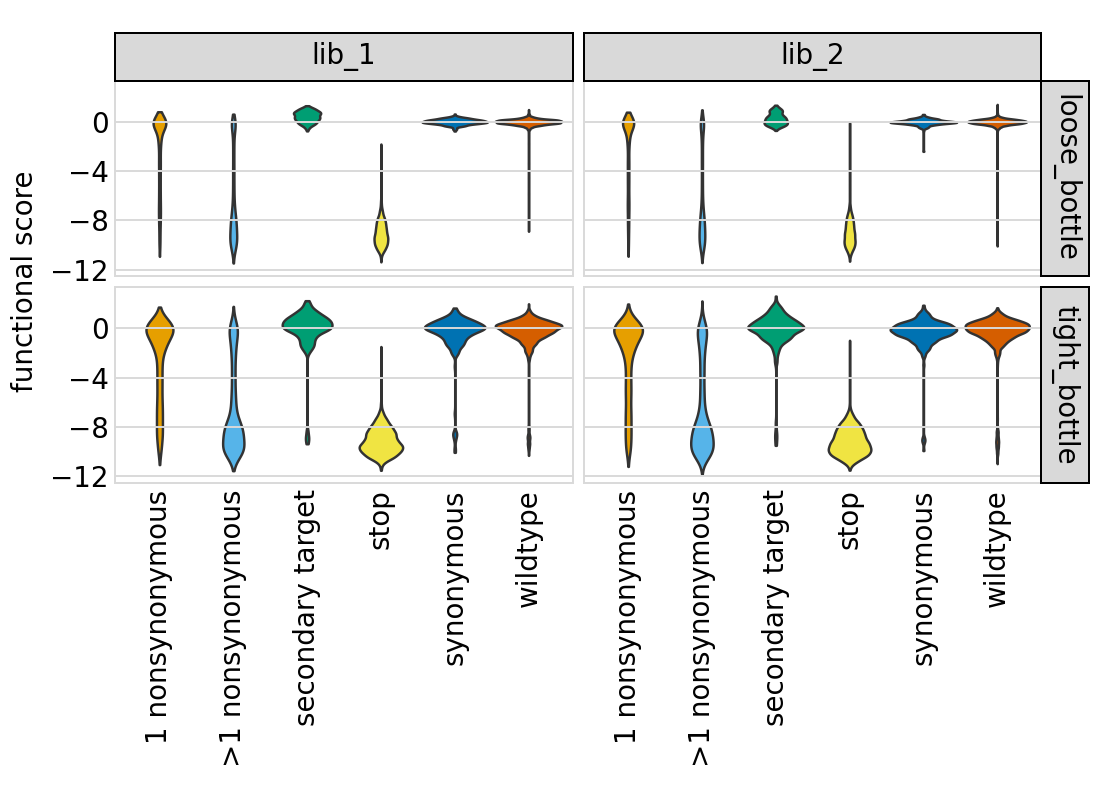
We can plot the distribution of the functional scores for variants. These plots are most informative if we classify variants by the “types” of mutations they have, which we do here using the CodonVariantTable.classifyVariants method, which adds a column called variant_class to the data frame. Note that we have to specify the primary target and how to classify non-primary targets:

func_scores = dms_variants.codonvarianttable.CodonVariantTable.classifyVariants(
    func_scores,
    primary_target=variants.primary_target,
    non_primary_target_class="secondary target",
)

(func_scores[["target", "codon_substitutions", "aa_substitutions", "variant_class"]])

	target	codon_substitutions	aa_substitutions	variant_class
0	primary_target_gene	ATC17CGA CGG29TGC	I17R R29C	>1 nonsynonymous
1	primary_target_gene	GCT7TCT AAA14GAT AAC20CGA	A7S K14D N20R	>1 nonsynonymous
2	primary_target_gene			wildtype
3	primary_target_gene	TTA18CTC		synonymous
4	primary_target_gene	CGT6GTA GAC22CAC	R6V D22H	>1 nonsynonymous
...	...	...	...	...
60863	secondary_target_3	secondary_target_3	secondary_target_3	secondary target
60864	secondary_target_3	secondary_target_3	secondary_target_3	secondary target
60865	secondary_target_3	secondary_target_3	secondary_target_3	secondary target
60866	secondary_target_3	secondary_target_3	secondary_target_3	secondary target
60867	secondary_target_3	secondary_target_3	secondary_target_3	secondary target

60868 rows × 4 columns

Now we use plotnine to plot the distributions of scores in ggplot2-like syntax, coloring by the variant class. This plot shows the expected behavior for different variant classes; for instance, stop codon variants tend to have low scores and synonymous variants tend to have wildtype-like (near 0) scores. As expected, there is more noise with a tighter bottleneck:

# NBVAL_IGNORE_OUTPUT

p = (
    ggplot(func_scores, aes("variant_class", "func_score"))
    + geom_violin(aes(fill="variant_class"))
    + ylab("functional score")
    + xlab("")
    + facet_grid("post_sample ~ library")
    + theme(
        figure_size=(2.75 * len(libs), 2 * len(bottlenecks)),
        axis_text_x=element_text(angle=90),
        panel_grid_major_x=element_blank(),  # no vertical grid lines
    )
    + scale_fill_manual(values=CBPALETTE[1:])
)

_ = p.draw(show=True)