Variants with deletion mutations

In some cases, you might want to include variants with in-frame codon-length deletions. There is an option to do this using --- as the codon gap character, and - as the resulting amino-acid gap character. Note that only codon-length in-frame deletions are allowed.

This notebook illustrates working with such variants.

Setup for analysis

Import Python modules / packages:

# NBVAL_IGNORE_OUTPUT

import random
import warnings

import pandas as pd

from plotnine import *

import dms_variants.codonvarianttable
import dms_variants.plotnine_themes
import dms_variants.simulate
from dms_variants.constants import CBPALETTE, CODONS_WITHGAP, CODONS_NOSTOP

Set parameters that define simulated data:

seed = 1  # random number seed
genelength = 30  # gene length in codons
libs = ["lib_1", "lib_2"]  # distinct libraries of gene
variants_per_lib = 500 * genelength  # variants per library
avgmuts = 2.0  # average codon mutations per variant
bclen = 16  # length of nucleotide barcode for each variant
variant_error_rate = 0.005  # rate at which variant sequence mis-called

Seed random number generator for reproducible output:

random.seed(seed)

Set pandas display options to show large chunks of Data Frames in this example:

pd.set_option("display.max_columns", 20)
pd.set_option("display.width", 500)

Hide warnings that clutter output:

warnings.simplefilter("ignore")

Set the gray grid plotnine theme defined in dms_variants.plotnine_themes as this gives a nice appearance for the plots:

theme_set(dms_variants.plotnine_themes.theme_graygrid())

Simulate library of variants

Simulate wildtype gene sequence:

geneseq = "".join(random.choices(CODONS_NOSTOP, k=genelength))
print(f"Wildtype gene of {genelength} codons:\n{geneseq}")

Wildtype gene of 30 codons:
AGATCCGTGATTCTGCGTGCTTACACCAACTCACGGGTGAAACGTGTAATCTTATGCAACAACGACTTACCTATCCGCAACATCCGGCTG

Generate a CodonVariantTable using simulate_CodonVariantTable function:

variants = dms_variants.simulate.simulate_CodonVariantTable(
    geneseq=geneseq,
    bclen=bclen,
    library_specs={
        lib: {"avgmuts": avgmuts, "nvariants": variants_per_lib} for lib in libs
    },
    seed=seed,
    allowgaps=True,
)

We can get basic information about the CodonVariantTable, such as the sites, wildtype codons, and wildtype amino acids. Below we do this for the first few sites:

variants.sites[:5]

[1, 2, 3, 4, 5]

list(variants.codons[r] for r in variants.sites[:5])

['AGA', 'TCC', 'GTG', 'ATT', 'CTG']

list(variants.aas[r] for r in variants.sites[:5])

['R', 'S', 'V', 'I', 'L']

The different libraries in the table:

variants.libraries

['lib_1', 'lib_2']

Here is the data frame that contains all of the information on the barcoded variants (just looking at the first few lines)

variants.barcode_variant_df.head(n=6)

	library	barcode	variant_call_support	codon_substitutions	aa_substitutions	n_codon_substitutions	n_aa_substitutions
0	lib_1	AAAAAACTAAAAGTCG	2	CGT15AGC ATC25GAA	R15S I25E	2	2
1	lib_1	AAAAACAATGCCGCAT	1	ACC9TCG TTA18TAC	T9S L18Y	2	2
2	lib_1	AAAAACAGACCTACAA	1	TCC2CCG TAC8TTC	S2P Y8F	2	2
3	lib_1	AAAAACCGTGGTTCTT	1	AGA1GAC CCT24GGC	R1D P24G	2	2
4	lib_1	AAAAACTCTATCTCAT	1	CTG5GTA GCT7TGG TCA11ACG CGG29CTG	L5V A7W S11T R29L	4	4
5	lib_1	AAAAACTTGAGCATGA	6	GTG3TCT GCT7TGG TAC8AAT TGC19TGA GAC22AGG AAC2...	V3S A7W Y8N C19* D22R N27D	6	6

Analyze library composition

A CodonVariantTable has methods for summarizing and plotting properties of the barcoded variants. These methods can be used to analyze the barcoded variants themselves, or to analyze the frequency (or counts) of variants in the library in samples that have undergone some type of selection.

We have not yet added counts of the variants in any specific samples, so we just analyze the composition of the variant library itself. This is done by setting samples=None in the method calls below.

Number of variants in each library:

variants.n_variants_df(samples=None)

	library	sample	count
0	lib_1	barcoded variants	15000
1	lib_2	barcoded variants	15000
2	all libraries	barcoded variants	30000

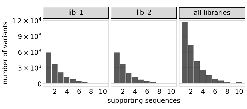
Plot distribution of variant call supports, grouping together all variants with support \(\ge 8\):

# NBVAL_IGNORE_OUTPUT

p = variants.plotVariantSupportHistogram(max_support=10)
p = p + theme(panel_grid_major_x=element_blank())  # no vertical grid lines
_ = p.draw(show=True)

The set of valid barcodes for each library:

for lib in libs:
    print(f"First few barcodes for library {lib}:")
    print(sorted(variants.valid_barcodes(lib))[:3])

First few barcodes for library lib_1:
['AAAAAACTAAAAGTCG', 'AAAAACAATGCCGCAT', 'AAAAACAGACCTACAA']
First few barcodes for library lib_2:
['AAAAAAACCCAGACTT', 'AAAAAACATCCGATCC', 'AAAAAACCTTCTGCCG']

Plot the number of amino-acid mutations per variant:

# NBVAL_IGNORE_OUTPUT

p = variants.plotNumMutsHistogram("aa", samples=None)
p = p + theme(panel_grid_major_x=element_blank())  # no vertical grid lines
_ = p.draw(show=True)

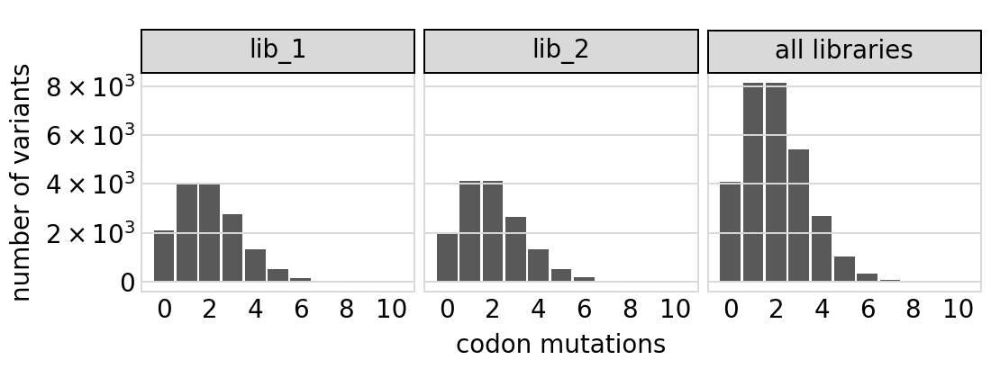
Number of codon mutations per variant:

# NBVAL_IGNORE_OUTPUT

p = variants.plotNumMutsHistogram("codon", samples=None)
p = p + theme(panel_grid_major_x=element_blank())  # no vertical grid lines
_ = p.draw(show=True)

Average number of codon mutations per variant of each type of mutation. We make these plots for: 1. Just single-mutant and wildtype variants 2. For all variants

# NBVAL_IGNORE_OUTPUT

for mut_type in ["single", "all"]:
    p = variants.plotNumCodonMutsByType(mut_type, samples=None, heightscale=1.5)
    p = p + theme(panel_grid_major_x=element_blank())  # no vertical grid lines
    _ = p.draw(show=True)

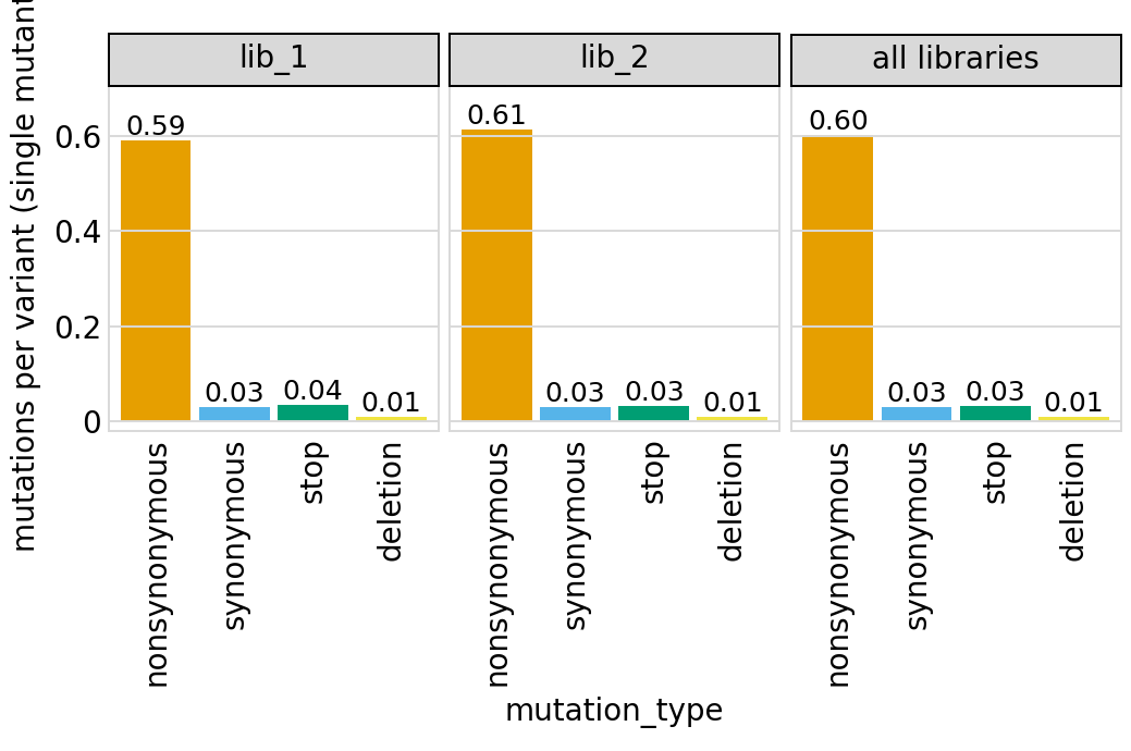
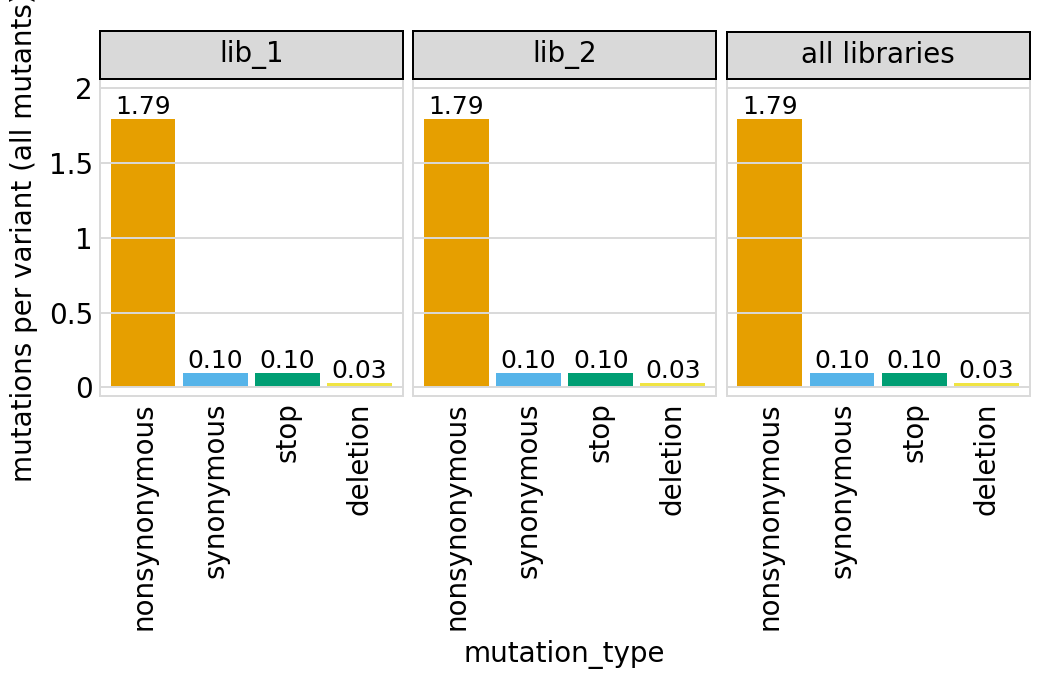
Here are the numerical data in the plots above:

variants.numCodonMutsByType("single", samples=None).round(3)

	library	sample	mutation_type	num_muts_count	count	number
0	lib_1	barcoded variants	nonsynonymous	3611	6112	0.591
1	lib_1	barcoded variants	synonymous	194	6112	0.032
2	lib_1	barcoded variants	stop	215	6112	0.035
3	lib_1	barcoded variants	deletion	56	6112	0.009
4	lib_2	barcoded variants	nonsynonymous	3746	6114	0.613
5	lib_2	barcoded variants	synonymous	188	6114	0.031
6	lib_2	barcoded variants	stop	196	6114	0.032
7	lib_2	barcoded variants	deletion	69	6114	0.011
8	all libraries	barcoded variants	nonsynonymous	7357	12226	0.602
9	all libraries	barcoded variants	synonymous	382	12226	0.031
10	all libraries	barcoded variants	stop	411	12226	0.034
11	all libraries	barcoded variants	deletion	125	12226	0.010

variants.numCodonMutsByType("all", samples=None).round(3)

	library	sample	mutation_type	num_muts_count	count	number
0	lib_1	barcoded variants	nonsynonymous	26917	15000	1.794
1	lib_1	barcoded variants	synonymous	1476	15000	0.098
2	lib_1	barcoded variants	stop	1457	15000	0.097
3	lib_1	barcoded variants	deletion	445	15000	0.030
4	lib_2	barcoded variants	nonsynonymous	26919	15000	1.795
5	lib_2	barcoded variants	synonymous	1485	15000	0.099
6	lib_2	barcoded variants	stop	1425	15000	0.095
7	lib_2	barcoded variants	deletion	458	15000	0.031
8	all libraries	barcoded variants	nonsynonymous	53836	30000	1.795
9	all libraries	barcoded variants	synonymous	2961	30000	0.099
10	all libraries	barcoded variants	stop	2882	30000	0.096
11	all libraries	barcoded variants	deletion	903	30000	0.030

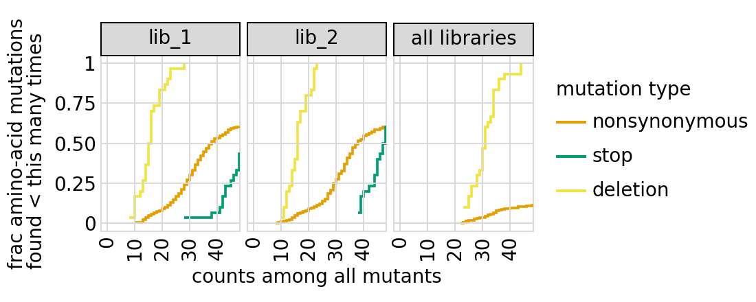
Examine how well amino-acid mutations are sampled in the library by looking at the fraction of mutations seen <= some number of times. Here we do that for amino- acid mutations, making separate plots for single mutants and all mutants:

# NBVAL_IGNORE_OUTPUT

for variant_type in ["single", "all"]:
    p = variants.plotCumulMutCoverage(variant_type, mut_type="aa", samples=None)
    _ = p.draw(show=True)

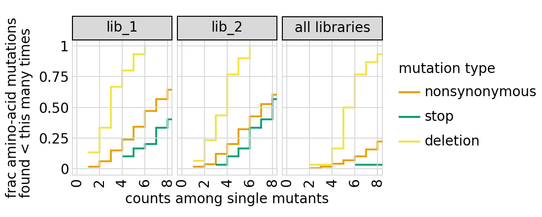
We can also get the numerical information plotted above (here for single mutants only):

variants.mutCounts("single", "aa", samples=None).head(n=5)

	library	sample	mutation	count	mutation_type	site
0	lib_1	barcoded variants	T9L	24	nonsynonymous	9
1	lib_1	barcoded variants	A7R	21	nonsynonymous	7
2	lib_1	barcoded variants	R1L	21	nonsynonymous	1
3	lib_1	barcoded variants	N10L	20	nonsynonymous	10
4	lib_1	barcoded variants	N27S	20	nonsynonymous	27

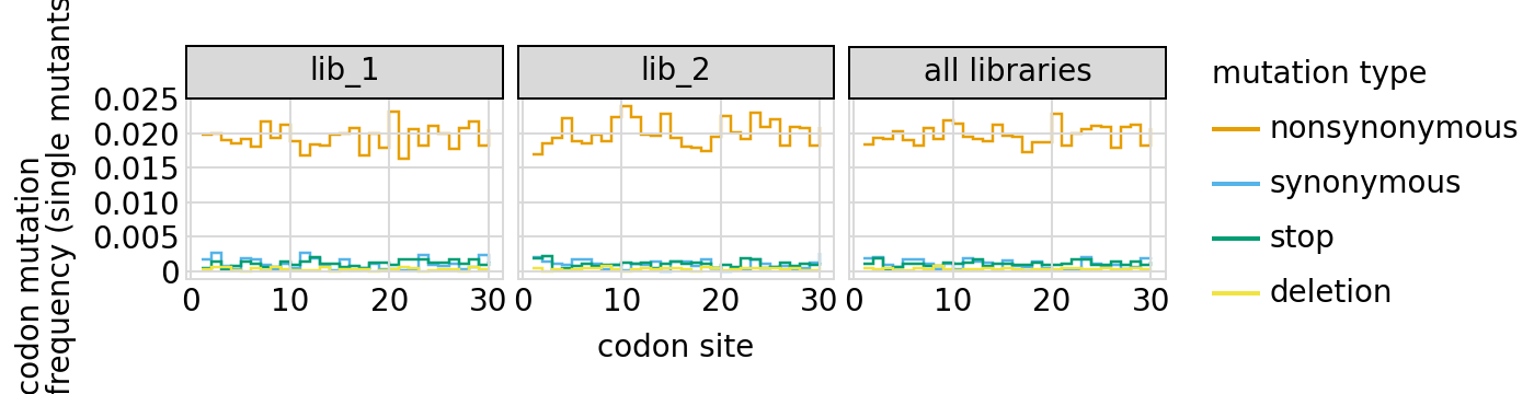
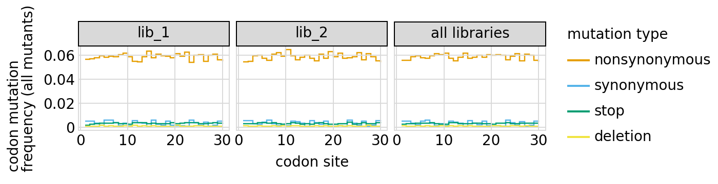
Here are the frequencies of mutations along the gene, looking both at single mutants and all mutants:

# NBVAL_IGNORE_OUTPUT

for variant_type in ["single", "all"]:
    p = variants.plotMutFreqs(variant_type, "codon", samples=None)
    _ = p.draw(show=True)

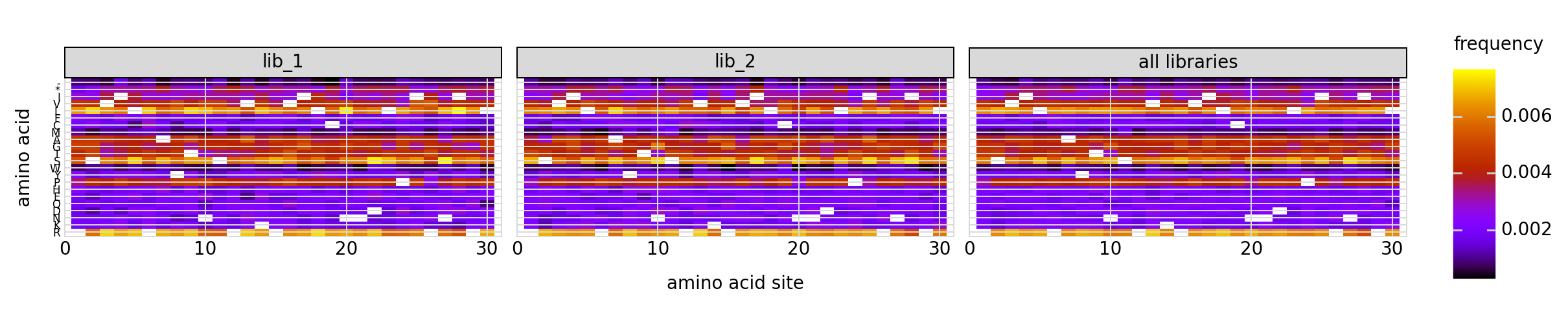
We can also look at mutation frequencies in a heat-map form:

p = variants.plotMutHeatmap("all", "aa", samples=None)
_ = p.draw(show=True)