Fraction surviving
Overview
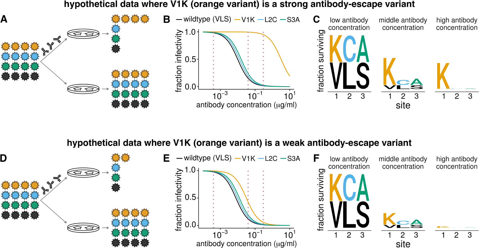
In some cases, you might subject a deep mutational scanning library to a harsh selection that purges most mutations. An example of such an experiment is selecting a virus library with a monoclonal antibody – most variants will be inactivated by the antibody, but those with mutations in the epitope will survive. If the experiment measures the fraction of the entire library that survives the selection as well as using sequencing to identify the frequencies of each mutation among the surviving variants, then it is possible to compute the fraction of variants with each mutation that survive the selection. This quantity is expected to range from zero (if all variants with a specific mutation are inactivated) to one (if all variants with a specific mutation survive the selection). An example of hypothetical fraction surviving data for such an experiment are in Fig. 7.

Fig. 7 Quantifying the fraction of virions with each mutation that escape antibody neutralization. This figure shows hypothetical data for four viral variants: wildtype and three mutants. (A) Virions with the V1K mutation (orange) completely survive an antibody concentration where most other virions are neutralized. (B) This resistance is manifested by a large shift in V1K’s neutralization curve. (C) For each dotted vertical line drawn through the neutralization curves in (B), we calculate the fraction of virions with that mutation that survive the antibody, and indicate this fraction by the height of the letter corresponding to that amino acid at that site. (D-F) Similar data to the first three panels, but now V1K has only a small antigenic effect, and so only modestly increases the fraction of virions that survive antibody treatment.
The dms_tools2 software contains programs to estimate the fraction of each mutation surviving from the overall fraction of the library that survives the selection and the deep sequencing data. Specifically, you can make these estimates using dms2_batch_fracsurvive, which in turn calls dms2_fracsurvive. These programs create visualizations of the results, and you can also visualize the fraction surviving with dms2_logoplot.
Definition of fraction surviving
This definition of the fraction surviving was originally introduced in Doud et al (2018).
We use \(F_{r,x}\) to denote the fraction of variants with character \(x\) (e.g., an amino acid) at site \(r\) that survive the selection.
In order to calculate \(F_{r,x}\), we need three pieces of information:
The overall fraction of the entire library that survives the selection. We will denote this quantity as \(\gamma\), and it should range from zero to one. For instance, \(\gamma\) might be calculated by using qPCR to determine the number of virions that infect cells in the presence of antibody versus the number that infect cells in the absence of antibody – the ratio of these two numbers would be the overall fraction of the entire library the survives the selection. You could also compute \(\gamma\) directly from deep-sequencing if your library contains some internal control variant that you know will not be affected by the selection (e.g., a variant with a totally orthogonal envelope protein that is not recognized by the antibody).
The number of deep sequencing counts of each character \(x\) at each site \(r\) in both the selected (e.g., antibody neutralized) and mock-selected samples. Denote these quantities as \(n_{r,x}^{\rm{selected}}\) and \(n_{r,x}^{\rm{mock}}\), respectively. Also define variables that give the total number of counts at each site for each condition as \(N_r^{\rm{selected}} = \sum_x n_{r,x}^{\rm{selected}}\) and \(N_r^{\rm{mock}} = \sum_x n_{r,x}^{\rm{mock}}\).
Given these pieces of information, the estimated fraction of variants in the selected and mock-selected libraries that contain character \(x\) at site \(r\) are calculated as:
where \(A\) is the number of characters (e.g., 20 for amino acids), \(P > 0\) is a pseudocount that is added to each observed count (specified by --pseudocount option to dms2_fracsurvive / dms2_batch_fracsurvive), and \(f_{r, \rm{selected}}\) and \(f_{r, \rm{mock}}\) are defined so that the pseudocount is scaled up for the library (mock or selected) with higher depth at site \(r\):
The reason for scaling the pseudocount by library depth is that the mock and selected libraries may often be sequenced at different depths.
If the same pseudocount is added to both, then the relative frequencies of mutations will be systematically different than one even if the relative counts for the wildtype and mutant amino acid are the same in both two conditions.
Scaling the pseudocounts by the ratio of depths fixes this problem.
If you are using --chartype of codon_to_aa, the counts for amino acids are aggregated before doing the calculations above.
If the mutation has no effect on whether or not a variant survives the selection, then we expect \(\rho_{r,x}^{\rm{selected}} = \rho_{r,x}^{\rm{mock}}\). On the other hand, if the mutation makes the variant more likely to survive the selection, then we expected \(\rho_{r,x}^{\rm{selected}} > \rho_{r,x}^{\rm{mock}}\). If the only variants that survive have the mutation, then we expect \(\rho_{r,x}^{\rm{selected}} = 1\) and the total fraction of the library \(\gamma\) that survives to just be equal to the unselected frequency of this mutation, \(\gamma = \rho_{r,x}^{\rm{mock}}\). More generally, the fraction of variants with mutation of \(r\) to \(x\) that survive the selection is
It is this quantity \(F_{r,x}\) that is reported by dms2_fracsurvive / dms2_batch_fracsurvive as the fraction of variants with the mutation surviving the selection (denoted as mutfracsurvive). Note that this quantity is calculated for the wildtype character at each site as well as all mutant characters.
In addition, these programs report two site-wise measures. These measures are calculated over all non-wildtype characters at each site:
The avgfracsurvive which is simply the average over all non-wildtype characters of the mutfracsurvive values at a site. If some mutfracsurvive values are NaN (which can happen if you use the
--mincountsoption), they are not included in the average.The maxfracsurvive which is simply the maximum mutfracsurvive over all non-wildtype characters at a site.
Fraction surviving above average
In the section above, \(F_{r,x}\) is defined in Equation (30) as the fraction of variants that survive given that they have the mutation of site \(r\) to \(x\). Note also that \(\gamma\) is the total fraction of the library that survives selection, or equivalently the average fraction that survives weighted over the variant frequencies.
In some cases, it is more useful to show that average fraction of variants that survive above this library average. To do this, we calculate the average fraction that survives above average as
If you call dms2_fracsurvive or dms2_batch_fracsurvive with the --aboveavg yes option then all results use these \(F_{r,x}^{\rm{aboveavg}}\) in place of \(F_{r,x}\) values.
The distinction is as follows.
If you want your results to reflect the average fraction of variants with each mutation that survive, then use the default --aboveavg no option.
In this case, you expect the fraction surviving to be > 0 for most variants, since a bit of your library probably gets through the selection even without an advantageous mutation.
On the other hand, if you just want to look for mutations that are enhancing how variants perform above the average, then use the --aboveavg yes option.
Then you only see fraction surviving > 0 for variants that are favored during the selection – but the quantitative values of this fraction surviving are no longer directly interpretable as the true fraction surviving, since they are in reference to the library average baseline.
Error correction
You can optionally correct for the potential inflation of some counts by sequencing errors by using the --err option to dms2_fracsurvive / dms2_batch_fracsurvive.
To do this, you should use some control where the only mutations will come from sequencing / library-prep-induced errors that are presumed to occur at the same rate as the actual samples being analyzed.
Typically, this would be deep sequencing of a wildtype control.
With an error control, the counts are adjusted as follows. Let \(n_{r,x}\) be the counts for character \(x\) at site \(r\) in the mock or selected sample. Let \(n^{\rm{err}}_{r,x}\) be the number of counts of \(x\) at site \(r\) in the error control. Define
When \(x \ne \operatorname{wt}\left(r\right)\) then \(\epsilon_{r,x}\) is the rate of errors to \(x\) at site \(r\), and when \(x = \operatorname{wt}\left(r\right)\) then \(\epsilon_{r,x}\) is one minus the rate of errors away from the wildtype at site \(r\).
We then adjust observed counts \(n_{r,x}\) to the error-corrected counts \(\hat{n}_{r,x}\) by
These adjusted counts are then used in place of the un-adjusted counts in Equation (29) above.
Programs and examples
The dms_tools2 software contains programs to calculate the fraction of each mutation surviving:
dms2_fracsurvive estimates the fraction surviving from counts files and the overall library fractiont that survives.
dms2_batch_fracsurvive runs dms2_fracsurvive on a set of samples and summarizes the results. It is generally easier to use dms2_batch_fracsurvive rather than runnning dms2_fracsurvive directly.
dms2_logoplot can be used to create logo plots that visualize the fraction surviving.
Here are some example analyses:

