Amino-acid preferences
Overview
A common goal of a deep mutational scanning experiment is to estimate the effect of every amino-acid mutation on a protein’s function. For instance, you might want to assess how each mutation to a viral protein affects the virus’s ability to replicate in cell-culture.
One way to quantify the effects of mutations is in terms of the preference of each site in the protein for each possible amino acid (Fig. 3). Essentially, highly preferred amino acids are enriched (or stay at the same frequency) after functional selection, whereas less preferred amino acid are depleted during functional selection.
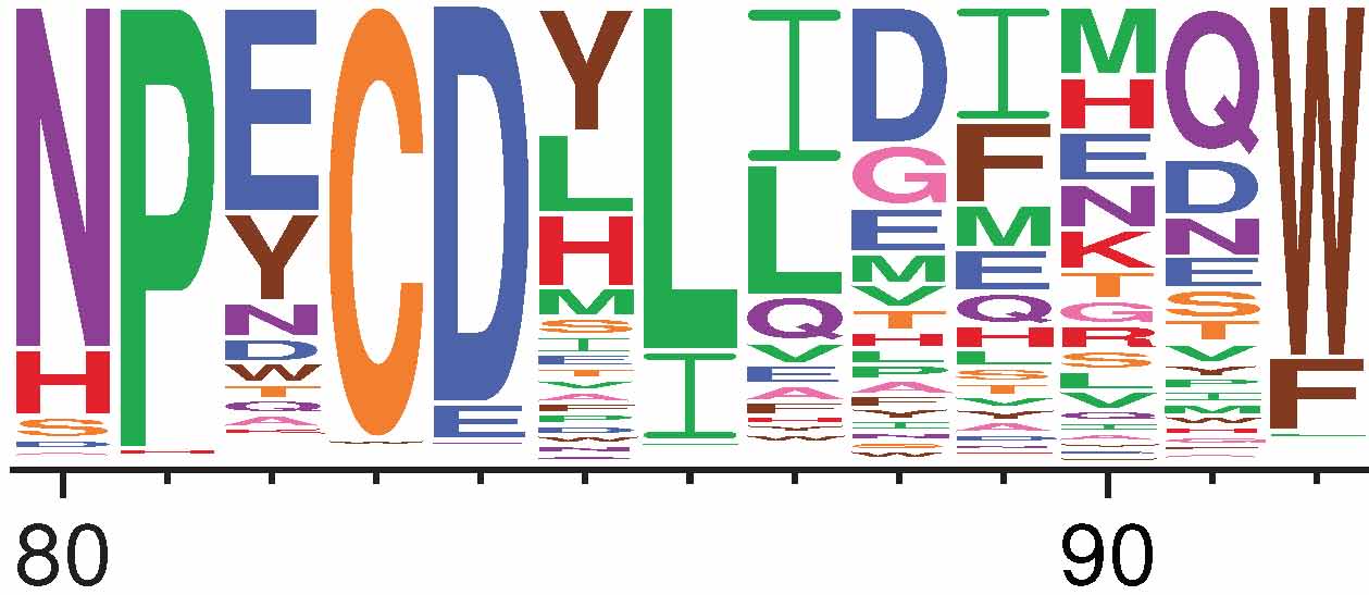
Fig. 3 Visualization of amino-acid preferences as created using dms2_logoplot. The height of each letter is proportional to the preference for that amino acid at that site. For instance, site 84 prefers the negatively charged amino acids aspartic acid (D) and glutamic acid (E), whereas site 86 prefers the hydrophobic amino acids leucine (L) and isoleucine (I).
A nice aspect of quantifying the effects of mutations in terms of amino-acid preferences is that the deep mutational scanning data can then be directly used to model evolution in nature (see Bloom (2014) and Bloom (2017)) using phylogenetics software like phydms. You can also estimate a stringency parameter that re-scales the preferences to better match the stringency of selection in nature (see Hilton et al (2017) and the Doud2016 example).
The dms_tools2 software contains programs to estimate the amino-acid preferences from the counts of mutations generated from the deep sequencing data. Typically you would want to estimate these preferences using dms2_batch_prefs, which in turn calls dms2_prefs. You then might visualize the preferences with dms2_logoplot and / or compare them to natural evolution using phydms.
The Examples include some analyses of this type of deep-sequencing data; for instance see the Doud2016 example.
What are amino-acid preferences?
Fig. 4 shows a schematic of how the amino-acid preferences are related to the counts of different mutations in deep mutational scanning. Specifically, we can imagine calculating the enrichment ratio of each mutation relative to wildtype both pre-selection and post-selection. Let \(E_{r,a}\) be the enrichment ratio for amino acid \(a\) at site \(r\). Then conceptually, the preference \(\pi_{r,a}\) for amino acid \(a\) at site \(r\) is simply obtained by normalizing all the enrichment ratios at that site: \(\pi_{r,a} = \frac{E_{r,a}}{\sum_{a'} E_{r,a'}}\). This is shown in Fig. 4.
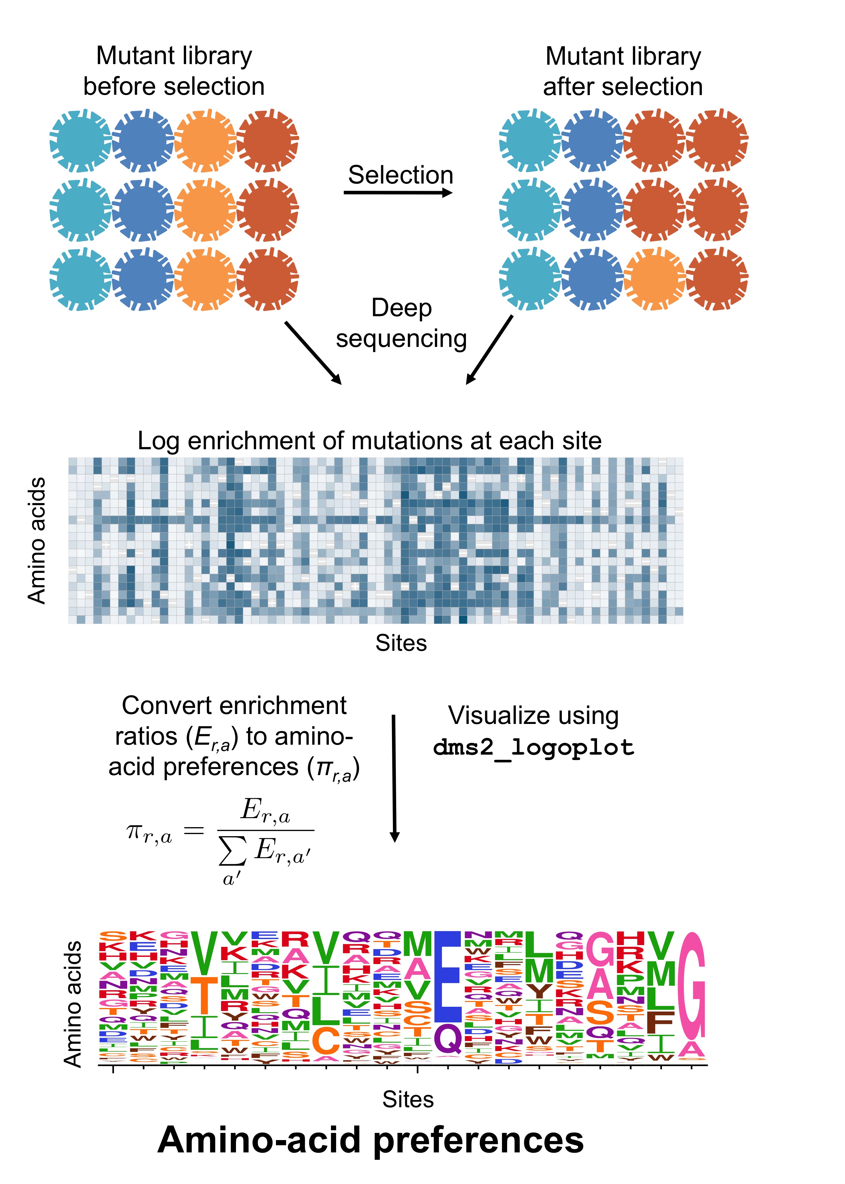
Fig. 4 Schematic of amino-acid preferences.
The experiment measures the frequency of each amino-acid before and after selection.
Imagine computing the enrichment of the mutation post-selection versus pre-selection.
These enrichment ratios can be displayed in a heat map.
However, dms2_prefs does not make these heat maps: instead it normalizes the enrichment of all amino acids at each site to calculate the preferences.
These can be displayed in a logo plot.
Note that the exact equation in this figure is used by dms2_prefs only if you use --method ratio and do not include any error-control counts.
If you use --method bayesian, a more sophisticated approach takes into account the statistical nature of the measurements.
If you use --err and then controls that estimate error rates are also taken into account.
However, it can be desirable to use a more statistically founded approach to estimate the same quantities, as described in Bloom (2015).
This more statistical treatment can be performed using the --method bayesian option to dms2_prefs.
You can also include controls that estimate the rate of errors in the samples.
You can specify controls that estimate the rates of errors using the --err option to dms2_prefs.
Typically these controls would come from deep-sequencing a wildtype library, where all apparent mutations are assumed to arise from deep sequencing errors rather than being true mutations.
These more sophisticated approaches estimate a quantity that asymptotically approaches the preferences estimated by the simple ratio approach if there are very large counts and no sequencing errors.
Should you use the bayesian or ratio method?
Two different approaches for estimating the preferences are implemented in dms2_prefs via the --method option: bayesian and ratio.
Generally, --method bayesian should be more accurate.
It also tends to handle the error controls (the --err option) better, particularly if the pre- and post-selection error controls are different.
So if you are using error-controls (particularly different pre- and post-selection ones), you should probably use this method.
The downside of --method bayesian is that it is fairly slow, and can lead to substantial run times of 5+ hours.
Note also that the priors used by --method bayesian assume that your mutagenesis method attempted to introduce all types of codon mutations at equal frequencies (e.g., NNN libraries).
If you favored some codons during library construction (e.g., NNK libraries), then the current priors will not be correct.
Using --method ratio is very fast.
If you do not have error controls, it will probably give fairly similar results to --method bayesian.
Its performance might decay if there are error controls, especially if the pre- and post-selection ones are different.
You can always run both methods and then compare the results (for instance, by using dms_tools2.plot.plotCorrMatrix function described in the Python API).
Programs and examples
The dms_tools2 software contains programs to estimate amino-acid preferences:
dms2_prefs estimates amino-acid preferences from counts files.
dms2_batch_prefs runs dms2_prefs on a set of samples and computes the correlations among samples. If you have multiple replicates, it is easier to use dms2_batch_prefs rather than runnning dms2_prefs directly.
dms2_logoplot can be used to create logo plots that visualize amino-acid preferences (potentially after re-scaling by a stringency parameter fit by phydms).
Note also that phydms can be used to perform phylogenetic analyses with the amino-acid preferences estimated using dms2_prefs / dms2_batch_prefs.
Here are some example analyses:
Algorithm to infer preferences when using --method bayesian
Here is a description of the algorithm that dms2_prefs uses to infer the site-specific preferences when you use --method bayesian.
This algorithm is detailed in Bloom (2015).
Definition of the site-specific preferences.
We assume each site \(r\) in our gene has a preference \(\pi_{r,x} \ge 0\) for each character \(x\), where the characters can be nucleotides, codons, or amino acids. The preferences are defined as follows: if \(\mu_{r,x}\) is the frequency of \(x\) at \(r\) in the mutant library pre-selection and \(f_{r,x}\) is the frequency of \(x\) in the library post-selection, then
This equation implies that \(1 = \sum_x \pi_{r,x}\).
The experimental data from deep sequencing.
We create mutant libraries such that each site \(r\) is potentially mutated from the wildtype identity to any of the other possible characters. We use deep sequencing to count the appearances of each character \(x\) at each site \(r\) in this mutant library; since this sequencing is performed prior to selection for gene function, we refer to it as pre-selection. Let \(N_r^{\textrm{pre}}\) be the total number of sequencing reads covering \(r\), and let \(n_{r,x}^{\textrm{pre}}\) be the number that report \(x\) (note that \(\mbox{$N_r^{\textrm{pre}}$}= \sum_x \mbox{$n_{r,x}^{\textrm{pre}}$}\)).
We impose an experimental selection on the mutant library with some biologically relevant pressure that favors some mutations and disfavor others. We then use deep sequencing to count the characters in this selected library; since this sequencing is performed after selection, we refer to it as post-selection. Let \(N_r^{\textrm{post}}\) be the total number of sequencing reads covering \(r\), and let \(n_{r,x}^{\textrm{post}}\) be the number that report \(x\) (note that \(\mbox{$N_r^{\textrm{post}}$}= \sum_x \mbox{$n_{r,x}^{\textrm{post}}$}\)).
We allow for the possibility that the deep sequencing is not completely accurate; for instance, perhaps some of the reads that report a mutant character reflect a sequencing error rather than a true mutation. The rates of such errors can be quantified by control sequencing of the unmutated gene, so that any counts at \(r\) of \(x \ne \mbox{$\operatorname{wt}\left(r\right)$}\) reflect sequencing errors. It is possible that the error rates for sequencing the pre-selection and post-selection libraries are different, as for instance would arise in sequencing an RNA virus for which the post-selection libraries must be reverse-transcribed to DNA prior to sequencing. Let \(N_r^{\textrm{err,pre}}\) be the total number of sequencing reads covering \(r\) in the pre-selection error control, and let \(n_{r,x}^{\textrm{err,pre}}\) be the number that report \(x\) (note that \(\mbox{$N_r^{\textrm{err,pre}}$}= \sum_x \mbox{$n_{r,x}^{\textrm{err,pre}}$}\)). Make similar definitions of \(N_r^{\textrm{err,post}}\) and \(n_{r,x}^{\textrm{err,post}}\) for the post-selection error control.
For notational compactness, we define vectors that contain the counts of all characters at each site \(r\) for each sample: \(\mbox{$\mathbf{n_r^{\textbf{pre}}}$}= \left(\cdots, \mbox{$n_{r,x}^{\textrm{pre}}$}, \cdots\right)\), \(\mbox{$\mathbf{n_r^{\textbf{post}}}$}= \left(\cdots, \mbox{$n_{r,x}^{\textrm{post}}$}, \cdots\right)\), \(\mbox{$\mathbf{n_r^{\textbf{err,pre}}}$}= \left(\cdots, \mbox{$n_{r,x}^{\textrm{err,pre}}$}, \cdots\right)\), and \(\mbox{$\mathbf{n_r^{\textbf{err,post}}}$}= \left(\cdots, \mbox{$n_{r,x}^{\textrm{err,post}}$}, \cdots\right)\).
Assumption that mutations and errors are rare.
The samples described above allow for the possibility of errors as well as the actual mutations. We assume that the the mutagenesis and error rates rate at each site are sufficiently low that most characters are wildtype, so for instance \(\mbox{$N_r^{\textrm{pre}}$}\sim \mbox{$n_{r,\operatorname{wt}\left(r\right)}^{\textrm{pre}}$}\gg \mbox{$n_{r,x}^{\textrm{pre}}$}\) for all \(x \ne \mbox{$\operatorname{wt}\left(r\right)$}\), and \(\mbox{$N_r^{\textrm{err,pre}}$}\sim \mbox{$n_{r,\operatorname{wt}\left(r\right)}^{\textrm{err,pre}}$}\gg \mbox{$n_{r,x}^{\textrm{err,pre}}$}\) for all \(x \ne \mbox{$\operatorname{wt}\left(r\right)$}\). This allows us to ignore as negligibly rare the possibility that the same site experiences both a mutation and an error in a single molecule, which simplifies the analysis below.
Actual frequencies and likelihoods of observing experimental data.
We have defined \(\mu_{r,x}\) and \(f_{r,x}\) as the frequencies of \(x\) at site \(r\) in the pre-selection and post-selection libraries, respectively. Also define \(\epsilon_{r,x}\) to be the frequency at which \(r\) is identified as \(x\) in sequencing the error control for the pre-selection library, and let \(\rho_{r,x}\) be the frequency at which \(r\) is identified as \(x\) in sequencing the error control for the post-selection library. For notational compactness, we define vectors of these frequencies for all characters at each site \(r\): \(\mbox{$\boldsymbol{\mathbf{\mu_r}}$}= \left(\cdots, \mu_{r,x}, \cdots\right)\), \(\mbox{$\boldsymbol{\mathbf{f_r}}$}= \left(\cdots, f_{r,x}, \cdots\right)\), \(\mbox{$\boldsymbol{\mathbf{\epsilon_r}}$}= \left(\cdots, \epsilon_{r,x}, \cdots\right)\), and \(\mbox{$\boldsymbol{\mathbf{\rho_r}}$}= \left(\cdots, \rho_{r,x}, \cdots\right)\). We also define \(\mbox{$\boldsymbol{\mathbf{\pi_r}}$}= \left(\cdots, \pi_{r,x}, \cdots\right)\). Note that Equation (1) implies that
where \(\circ\) is the Hadamard product.
Unless we exhaustively sequence every molecule in each library, the observed counts will not precisely reflect their actual frequencies in the libraries, since the deep sequencing only observes a sample of the molecules. If the deep sequencing represents a random sampling of a small fraction of a large library of molecules, then the likelihood of observing some specific set of counts will be multinomially distributed around the actual frequencies. So
where \(\operatorname{Multinomial}\) denotes the Multinomial distribution, \(\mbox{$\boldsymbol{\mathbf{\delta_r}}$}= \left(\cdots, \delta_{x, \operatorname{wt}\left(r\right)}, \cdots\right)\) is a vector for which the element corresponding to \(\operatorname{wt}\left(r\right)\) is one and all other elements are zero (\(\delta_{xy}\) is the Kronecker delta), and we have assumed that the probability that a site experiences both a mutation and an error is negligibly small. Similarly,
Priors over the unknown parameters.
We specify Dirichlet priors over the four parameter vectors for each site \(r\):
where \(\mathbf{1}\) is a vector of ones, \(\mathcal{N}_x\) is the number of characters (i.e. 64 for codons, 20 for amino acids, 4 for nucleotides), the \(\alpha\) parameters (i.e. \(\alpha_{\pi}\), \(\alpha_{\mu}\), \(\alpha_{\epsilon}\), and \(\alpha_{\rho}\)) are scalar concentration parameters with values \(> 0\) specified by the user, and the \(\mathbf{a_r}\) vectors have entries \(> 0\) that sum to one.
We specify the prior vectors \(\mathbf{a_{r,\mu}}\), \(\mathbf{a_{r,\epsilon}}\), and \(\mathbf{a_{r,\rho}}\) in terms of the average per-site mutation or error rates over the entire library.
Our prior assumption is that the rate of sequencing errors depends on the number of nucleotides being changed – for nucleotide characters all mutations have only one nucleotide changed, but for codon characters there can be one, two, or three nucleotides changed. Specifically, the average per-site error rate for mutations with \(m\) nucleotide changes \(\overline{\epsilon_m}\) and \(\overline{\rho_m}\) in the pre-selection and post-selection controls, respectively, are defined as
where \(L\) is the number of sites with deep mutational scanning data, \(r\) ranges over all of these sites, \(x\) ranges over all characters (nucleotides or codons), and \(D_{x,\operatorname{wt}\left(r\right)}\) is the number of nucleotide differences between \(x\) and the wildtype character \(\operatorname{wt}\left(r\right)\). Note that \(1 = \sum\limits_m \overline{\epsilon_m} = \sum\limits_m \overline{\rho_m}\).
Given these definitions, we define the prior vectors for the error rates as
where \(\mathcal{C}_m\) is the number of mutant characters with \(m\) changes relative to the wildtype (so for nucleotides \(\mathcal{C}_0 = 1\) and \(\mathcal{C}_1 = 3\), while for codons \(\mathcal{C}_0 = 1\), \(\mathcal{C}_1 = 9\), \(\mathcal{C}_2 = \mathcal{C}_3 = 27\)) and \(\delta_{xy}\) is again the Kronecker delta.
Our prior assumption is that the mutagenesis is done so that all mutant characters are introduced at equal frequency – note that this assumption is only true for codon characters if the mutagenesis is done at the codon level. In estimating the mutagenesis rate, we need to account for the facts that the observed counts of non-wildtype characters in the pre-selection mutant library will be inflated by the error rate represented by \(\overline{\epsilon_m}\). We therefore estimate the per-site mutagenesis rate as
Note that a value of \(\overline{\mu} \le 0\) would suggest that mutations are no more prevalent (or actually less prevalent) in the pre-selection mutant library then the pre-selection error control. Such a situation would violate the assumptions of the experiment, and so the algorithm will halt if this is the case. The prior vector for the mutagenesis rate is then
Currently, dms2_prefs is designed to work only for the case where the
deep sequencing counts are for codon
characters \(x\), but that we want to determine the preferences
\(\pi_{r,a}\) for amino-acid characters \(a\).
(This is what the --chartype codon_to_aa option means in dms2_prefs).
This situation occurs
if the mutant library is generated by
introducing all possible codon mutations at each site and we are
assuming that all selection acts at the protein level (so all codons
for the same amino-acid should have the same preference). In this
case, we define the vector-valued function \(\mathbf{A}\) to map
from codons to amino acids, so that
where \(\mathbf{w}\) is a 64-element vector giving the values for each codon \(x\), \(\mathbf{A}\left(\mathbf{w}\right)\) is a 20-element vector giving the values for each amino acid \(a\) (or a 21-element vector if stop codons are considered a possible amino-acid identity), and \(\mathcal{A}\left(x\right)\) is the amino acid encoded by codon \(x\). The parameter vectors \(\boldsymbol{\mathbf{\pi_r}}\), \(\boldsymbol{\mathbf{\mu_r}}\), \(\boldsymbol{\mathbf{\epsilon_r}}\), and \(\boldsymbol{\mathbf{\rho_r}}\) are then all of length 20 (or 21) for the amino acid vectors. The first of these vectors is still a symmetric Dirichlet, and the priors for the remaining three are \(\mathbf{A}\left(\mbox{$\boldsymbol{\mathbf{a_{r,\mu}}}$}\right)\), \(\mathbf{A}\left(\mbox{$\boldsymbol{\mathbf{a_{r,\epsilon}}}$}\right)\), and \(\mathbf{A}\left(\mbox{$\boldsymbol{\mathbf{a_{r,\rho}}}$}\right)\) for the \(\boldsymbol{\mathbf{a_{r,\mu}}}\), \(\boldsymbol{\mathbf{a_{r,\epsilon}}}\), and \(\boldsymbol{\mathbf{a_{r,\rho}}}\) vectors defined for codons immediately above. The likelihoods are computed by similarly transforming the count vectors in Equations (3), (6), (4), and (5) to \(\mathbf{A}\left(\mbox{$\mathbf{n_r^{\textbf{pre}}}$}\right)\), \(\mathbf{A}\left(\mbox{$\mathbf{n_r^{\textbf{post}}}$}\right)\), \(\mathbf{A}\left(\mbox{$\mathbf{n_r^{\textbf{err,pre}}}$}\right)\), and \(\mathbf{A}\left(\mbox{$\mathbf{n_r^{\textbf{err,post}}}$}\right)\).
Inferring the preferences by MCMC.
Given the sequencing data and the parameters that specify the priors, the posterior probability of any given set of the parameters \(\boldsymbol{\mathbf{\pi_r}}\), \(\boldsymbol{\mathbf{\mu_r}}\), \(\boldsymbol{\mathbf{\epsilon_r}}\), and \(\boldsymbol{\mathbf{\rho_r}}\) is given by the product of Equations (3), (6), (4), (5), (7), (8), (9), and (10). We use MCMC implemented by PyStan to sample from this posterior distribution. We monitor for convergence of the sampling of the site-specific preferences by running four chains, and ensuring that the mean over all \(\pi_{r,x}\) values of the potential scale reduction statistic \(\hat{R}\) of GelmanRubin1992 is \(\le 1.1\) and that the mean effective sample size is \(\ge 100\), or that \(\hat{R} \le 1.15\) and the effective sample size is \(\ge 300\). We repeatedly increase the number of steps until convergence occurs. The inferred preferences are summarized by the posterior mean and median-centered 95% credible interval for each \(\pi_{r,x}\).
Formula to calculate preferences with --method ratio
When using --method ratio in dms2_prefs, we calculate the preferences as
where \(\phi_{r,a}\) is the enrichment ratio of character \(a\) relative to wildtype after selection.
The actual definition of these enrichment ratios is somewhat complex due to the need to correct for errors and add a pseudocount. We have 4 sets of counts:
pre: pre-selection counts
post: post-selection counts
errpre: error-control for pre-selection counts
errpost: error-control for post-selection counts
For each set of counts \(s\), let \(N_r^s\) (e.g., \(N_r^{pre}\)) denote the total counts for this sample at site \(r\), and let \(n_{r,a}^{s}\) (e.g., \(n_{r,a}^{pre}\)) denote the counts at that site for character \(a\).
Because some of the counts are low, we add a pseudocount
\(P\) to each observation. Importantly, we need to scale
this pseudocount by the total depth for that sample at that site
in order to avoid systematically estimating different frequencies
purely as a function of sequencing depth, which will bias
the preference estimates.
Therefore, given the pseudocount value \(P\) defined via the
--pseudocount argument to dms2_prefs, we calculate the
scaled pseudocount for sample \(s\) and site \(r\) as
This equation makes the pseudocount \(P\) for the lowest-depth sample, and scales up the pseodocounts for all other samples proportional to their depth.
With this pseudocount, the estimated frequency of character \(a\) at site \(r\) in sample \(s\) is
where \(A\) is the number of characters in the alphabet (e.g., 20 for amino acids without stop codons).
The error-corrected estimates of the frequency of character \(a\) before and after selection are then
where \(\delta_{a,\rm{wt}\left(r\right)}\) is the Kronecker-delta, equal to 1 if \(a\) is the same as the wildtype character \(\rm{wt}\left(r\right)\) at site \(r\), and 0 otherwise. We use the \(\max\) operator to ensure that even if the error-control frequency exceeds the actual estimate, our estimated frequency never drops below the pseudocount over the depth of the uncorrected sample.
Given these definitions, we then simply calculate the enrichment ratios as
In the case where we are not using any error-controls, then we simply set \(f_{r,\rm{wt}}^{errpre} = f_{r,\rm{wt}}^{errpost} = \delta_{a,\rm{wt}\left(r\right)}\).